Difference of Gaussians
In imaging science, difference of Gaussians (DoG) is a feature enhancement algorithm that involves the subtraction of one Gaussian blurred version of an original image from another, less blurred version of the original. In the simple case of grayscale images, the blurred images are obtained by convolving the original grayscale images with Gaussian kernels having differing width (standard deviations). Blurring an image using a Gaussian kernel suppresses only high-frequency spatial information. Subtracting one image from the other preserves spatial information that lies between the range of frequencies that are preserved in the two blurred images. Thus, the DoG is a spatial band-pass filter that attenuates frequencies in the original grayscale image that are far from the band center.[1]
Formulation

Let denote the radial Gaussian function with mean and variance , i.e., the multivariate Gaussian function with mean and covariance . More explicitly, we have
The difference of Gaussians with variances is the kernel function
obtained by subtracting the higher-variance Gaussian from the lower-variance Gaussian. The difference of Gaussian operator is the convolutional operator associated with this kernel function. So given an n-dimensional grayscale image , the difference of Gaussians of the image is the n-dimensional image
Because convolution is bilinear, convolving against the difference of Gaussians is equivalent to applying two different Gaussian blurs and then taking the difference. In practice, this is faster because Gaussian blur is a separable filter.
Approximation
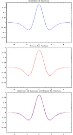
The difference of Gaussians can be thought of as an approximation of the Mexican hat kernel function used for the Laplacian of the Gaussian operator. The key observation is that the family of Gaussians is the fundamental solution of the heat equation
The left-hand side can be approximated by the difference quotient
Meanwhile, the right-hand side is precisely the Laplacian of the Gaussian function. Note that the Laplacian of the Gaussian can be used as a filter to produce a Gaussian blur of the Laplacian of the image because by standard properties of convolution. The relationship between the difference of Gaussians operator and the Laplacian of the Gaussian operator is explained further in Appendix A in Lindeberg (2015).[2]
Details and applications


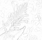
As a feature enhancement algorithm, the difference of Gaussians can be utilized to increase the visibility of edges and other detail present in a digital image. A wide variety of alternative edge sharpening filters operate by enhancing high frequency detail, but because random noise also has a high spatial frequency, many of these sharpening filters tend to enhance noise, which can be an undesirable artifact. The difference of Gaussians algorithm removes high frequency detail that often includes random noise, rendering this approach one of the most suitable for processing images with a high degree of noise. A major drawback to application of the algorithm is an inherent reduction in overall image contrast produced by the operation.[1]
When utilized for image enhancement, the difference of Gaussians algorithm is typically applied when the size ratio of kernel (2) to kernel (1) is 4:1 or 5:1. In the example images, the sizes of the Gaussian kernels employed to smooth the sample image were 10 pixels and 5 pixels.
The algorithm can also be used to obtain an approximation of the Laplacian of Gaussian when the ratio of size 2 to size 1 is roughly equal to 1.6.[3] The Laplacian of Gaussian is useful for detecting edges that appear at various image scales or degrees of image focus. The exact values of sizes of the two kernels that are used to approximate the Laplacian of Gaussian will determine the scale of the difference image, which may appear blurry as a result.
Differences of Gaussians have also been used for blob detection in the scale-invariant feature transform (SIFT). In fact, the DoG as the difference of two Multivariate normal distribution has always a total null sum and convolving it with a uniform signal generates no response. It approximates well a second derivate of Gaussian (Laplacian of Gaussian) with K~1.6 and the receptive fields of ganglion cells in the retina with K~5. It may easily be used in recursive schemes and is used as an operator in real-time algorithms for blob detection and automatic scale selection.
More information
In its operation, the difference of Gaussians algorithm is believed to mimic how neural processing in the retina of the eye extracts details from images destined for transmission to the brain.[4] [5] [6]
See also
- Marr–Hildreth algorithm
- Treatment of the difference of Gaussians approach in blob detection.
- Blob detection
- Gaussian pyramid
- Scale space
References
- ↑ 1.0 1.1 "Molecular Expressions Microscopy Primer: Digital Image Processing – Difference of Gaussians Edge Enhancement Algorithm", Olympus America Inc., and Florida State University Michael W. Davidson, Mortimer Abramowitz
- ↑ Lindeberg, Tony (2015). "Image Matching Using Generalized Scale-Space Interest Points". Journal of Mathematical Imaging and Vision 52: 3–36. doi:10.1007/s10851-014-0541-0.
- ↑ D. Marr; E. Hildreth (29 February 1980). "Theory of Edge Detection". Proceedings of the Royal Society of London. Series B, Biological Sciences 207 (1167): 215–217. doi:10.1098/rspb.1980.0020. PMID 6102765. Bibcode: 1980RSPSB.207..187M. — A difference of Gaussians of any scale is an approximation to the laplacian of the Gaussian (see the entry for difference of Gaussians under Blob detection). However, Marr and Hildreth recommend the ratio of 1.6 because of design considerations balancing bandwidth and sensitivity. The url for this reference may only make the first page and abstract of the article available depending on if you are connecting through an academic institution or not.
- ↑ Christina Enroth-Cugell; J. G. Robson (1966). "The Contrast Sensitivity of Retinal Ganglion Cells of the Cat.". Journal of Physiology 187 (3): 517–552. doi:10.1113/jphysiol.1966.sp008107. PMID 16783910.
- ↑ Matthew J. McMahon; Orin S. Packer; Dennis M. Dacey (April 14, 2004). "The Classical Receptive Field Surround of Primate Parasol Ganglion Cells Is Mediated Primarily by a Non-GABAergic Pathway". Journal of Neuroscience 24 (15): 3736–3745. doi:10.1523/JNEUROSCI.5252-03.2004. PMID 15084653. PMC 6729348. http://www.jneurosci.org/content/jneuro/24/15/3736.full.pdf.
- ↑ Young, Richard (1987). "The Gaussian derivative model for spatial vision: I. Retinal mechanisms". Spatial Vision 2 (4): 273–293(21). doi:10.1163/156856887X00222. PMID 3154952.
Further reading
- Notes by Melisa Durmuş on Edge Detection and Gaussian related mathematics from the University of Edinburgh.
 |
