Differential equations, ordinary, approximate methods of solution of
Methods for obtaining analytical expressions (formulas) or numerical values which approximate to some degree of accuracy the required particular solution of a differential equation or of a system of equations for one or more values of the argument. The importance of approximate methods of solution of differential equations is due to the fact that exact solutions in the form of analytical expressions are only known for a few types of differential equations.
One of the oldest methods for the approximate solution of ordinary differential equations is their expansion into a Taylor series. In this method the solution of an equation
| <img align="absmiddle" border="0" src="https://www.encyclopediaofmath.org/legacyimages/d/d032/d032080/d0320801.png" /> |
with the initial condition
| <img align="absmiddle" border="0" src="https://www.encyclopediaofmath.org/legacyimages/d/d032/d032080/d0320802.png" /> |
is approximated by a partial sum of the Taylor series
| <img align="absmiddle" border="0" src="https://www.encyclopediaofmath.org/legacyimages/d/d032/d032080/d0320803.png" /> |
The derivatives <img align="absmiddle" border="0" src="https://www.encyclopediaofmath.org/legacyimages/d/d032/d032080/d0320804.png" /> are expressed in terms of <img align="absmiddle" border="0" src="https://www.encyclopediaofmath.org/legacyimages/d/d032/d032080/d0320805.png" /> and its partial derivatives:
| <img align="absmiddle" border="0" src="https://www.encyclopediaofmath.org/legacyimages/d/d032/d032080/d0320806.png" /> |
| <img align="absmiddle" border="0" src="https://www.encyclopediaofmath.org/legacyimages/d/d032/d032080/d0320807.png" /> |
etc. The error of the method is directly proportional to <img align="absmiddle" border="0" src="https://www.encyclopediaofmath.org/legacyimages/d/d032/d032080/d0320808.png" />. For large values of <img align="absmiddle" border="0" src="https://www.encyclopediaofmath.org/legacyimages/d/d032/d032080/d0320809.png" /> the error slowly tends to zero as <img align="absmiddle" border="0" src="https://www.encyclopediaofmath.org/legacyimages/d/d032/d032080/d03208010.png" />, while if the value of <img align="absmiddle" border="0" src="https://www.encyclopediaofmath.org/legacyimages/d/d032/d032080/d03208011.png" /> exceeds that of the convergence radius of the Taylor series, the error usually does not tend to zero as <img align="absmiddle" border="0" src="https://www.encyclopediaofmath.org/legacyimages/d/d032/d032080/d03208012.png" />. This fact, as well as the necessity for computing a large number of partial derivatives, strongly restricts the scope of applicability of the method. The method of expansion into a Taylor series as well as methods based on the expansion in series of a more general nature are commonly used to find an approximate solution in the form of an analytical expression. Methods applicable for this purpose also include the Chaplygin method, which involves differential inequalities, and the method of sequential approximation (cf. Sequential approximation, method of). These methods are mainly employed in theoretical investigations and are used only rarely to obtain numerical solutions of differential equations in practical computations.
Asymptotic methods for the approximate solution of differential equations based on separating the equation to be solved into principal terms and terms which are small as compared with principal terms are often employed in practical work. Small parameter methods (cf. Small parameter, method of the) for the equation <img align="absmiddle" border="0" src="https://www.encyclopediaofmath.org/legacyimages/d/d032/d032080/d03208013.png" /> may serve as an example. Asymptotic methods are used both to obtain analytical expressions approximating the solution and in the study of the qualitative behaviour of solutions.
In the most frequently used methods for obtaining a numerical solution of differential equations, the solution is sought in the form of a table of approximate values of the unknown function <img align="absmiddle" border="0" src="https://www.encyclopediaofmath.org/legacyimages/d/d032/d032080/d03208014.png" /> for several values of the argument <img align="absmiddle" border="0" src="https://www.encyclopediaofmath.org/legacyimages/d/d032/d032080/d03208015.png" /> in an interval <img align="absmiddle" border="0" src="https://www.encyclopediaofmath.org/legacyimages/d/d032/d032080/d03208016.png" />. For instance, consider the solution of an equation <img align="absmiddle" border="0" src="https://www.encyclopediaofmath.org/legacyimages/d/d032/d032080/d03208017.png" /> with initial condition <img align="absmiddle" border="0" src="https://www.encyclopediaofmath.org/legacyimages/d/d032/d032080/d03208018.png" /> on an interval <img align="absmiddle" border="0" src="https://www.encyclopediaofmath.org/legacyimages/d/d032/d032080/d03208019.png" /> under the assumption that the solution is to be computed for the argument values
| <img align="absmiddle" border="0" src="https://www.encyclopediaofmath.org/legacyimages/d/d032/d032080/d03208020.png" /> |
The quantities <img align="absmiddle" border="0" src="https://www.encyclopediaofmath.org/legacyimages/d/d032/d032080/d03208021.png" /> are called the nodes, while the magnitude <img align="absmiddle" border="0" src="https://www.encyclopediaofmath.org/legacyimages/d/d032/d032080/d03208022.png" /> is called the step; <img align="absmiddle" border="0" src="https://www.encyclopediaofmath.org/legacyimages/d/d032/d032080/d03208023.png" /> denotes the value of the approximate solution at the node <img align="absmiddle" border="0" src="https://www.encyclopediaofmath.org/legacyimages/d/d032/d032080/d03208024.png" />.
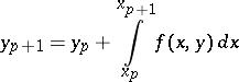
One of the simplest numerical methods — the Euler method — is based on an approximate computation of the integral term in the identity
| <img align="absmiddle" border="0" src="https://www.encyclopediaofmath.org/legacyimages/d/d032/d032080/d03208025.png" /> |
by quadratures, using the rectangle formula
| <img align="absmiddle" border="0" src="https://www.encyclopediaofmath.org/legacyimages/d/d032/d032080/d03208026.png" /> |
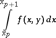
The truncation error of Euler's method is proportional to <img align="absmiddle" border="0" src="https://www.encyclopediaofmath.org/legacyimages/d/d032/d032080/d03208027.png" />. By approximating the integral
| <img align="absmiddle" border="0" src="https://www.encyclopediaofmath.org/legacyimages/d/d032/d032080/d03208028.png" /> | (1) |
by more exact quadrature formulas it is possible to obtain more exact numerical methods. For instance, if the trapezoidal formula is employed to approximate (1), then
| <img align="absmiddle" border="0" src="https://www.encyclopediaofmath.org/legacyimages/d/d032/d032080/d03208029.png" /> |
This equation is usually not directly solvable, e.g. for <img align="absmiddle" border="0" src="https://www.encyclopediaofmath.org/legacyimages/d/d032/d032080/d03208030.png" />. It may be solved by iteration methods, taking the value of <img align="absmiddle" border="0" src="https://www.encyclopediaofmath.org/legacyimages/d/d032/d032080/d03208031.png" /> obtained by Euler's method as an initial approximation. One iteration leads to the formulas:
| <img align="absmiddle" border="0" src="https://www.encyclopediaofmath.org/legacyimages/d/d032/d032080/d03208032.png" /> |
where
| <img align="absmiddle" border="0" src="https://www.encyclopediaofmath.org/legacyimages/d/d032/d032080/d03208033.png" /> |
and
| <img align="absmiddle" border="0" src="https://www.encyclopediaofmath.org/legacyimages/d/d032/d032080/d03208034.png" /> |
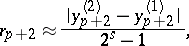
The error of these formulas is of the order <img align="absmiddle" border="0" src="https://www.encyclopediaofmath.org/legacyimages/d/d032/d032080/d03208035.png" />. They belong to the family of Runge–Kutta methods (cf. Runge–Kutta method). One familiar method of this type involves an error of the order <img align="absmiddle" border="0" src="https://www.encyclopediaofmath.org/legacyimages/d/d032/d032080/d03208036.png" />. Runge–Kutta methods are one-step methods, since it is sufficient to know <img align="absmiddle" border="0" src="https://www.encyclopediaofmath.org/legacyimages/d/d032/d032080/d03208037.png" /> — the value of the approximate solution in the previous step — to compute <img align="absmiddle" border="0" src="https://www.encyclopediaofmath.org/legacyimages/d/d032/d032080/d03208038.png" />. This is the reason why the Runge–Kutta methods may also be employed if the nodes are not equispaced — i.e. if the difference <img align="absmiddle" border="0" src="https://www.encyclopediaofmath.org/legacyimages/d/d032/d032080/d03208039.png" /> is not constant. In choosing the integration step, it is useful if some estimate of the step error of the method is available. This error can, e.g., be estimated by Richardson extrapolation: <img align="absmiddle" border="0" src="https://www.encyclopediaofmath.org/legacyimages/d/d032/d032080/d03208040.png" /> is computed twice, by two steps of length <img align="absmiddle" border="0" src="https://www.encyclopediaofmath.org/legacyimages/d/d032/d032080/d03208041.png" /> and one of length <img align="absmiddle" border="0" src="https://www.encyclopediaofmath.org/legacyimages/d/d032/d032080/d03208042.png" />; the values thus obtained are denoted by <img align="absmiddle" border="0" src="https://www.encyclopediaofmath.org/legacyimages/d/d032/d032080/d03208043.png" /> and <img align="absmiddle" border="0" src="https://www.encyclopediaofmath.org/legacyimages/d/d032/d032080/d03208044.png" />, respectively; the error in the step is
| <img align="absmiddle" border="0" src="https://www.encyclopediaofmath.org/legacyimages/d/d032/d032080/d03208045.png" /> |
where <img align="absmiddle" border="0" src="https://www.encyclopediaofmath.org/legacyimages/d/d032/d032080/d03208046.png" /> is the order of <img align="absmiddle" border="0" src="https://www.encyclopediaofmath.org/legacyimages/d/d032/d032080/d03208047.png" /> with respect to <img align="absmiddle" border="0" src="https://www.encyclopediaofmath.org/legacyimages/d/d032/d032080/d03208048.png" /> (for Euler's method <img align="absmiddle" border="0" src="https://www.encyclopediaofmath.org/legacyimages/d/d032/d032080/d03208049.png" />, for the trapezoidal formula <img align="absmiddle" border="0" src="https://www.encyclopediaofmath.org/legacyimages/d/d032/d032080/d03208050.png" />, etc.). Another method for estimating the step error is to obtain formulas of Runge–Kutta type with a control term which approximates the principal term of the step error of the method accurate up to small terms of higher orders. Also so-called implicit one-step methods have been developed and have been proved highly effective in certain classes of problems, but mainly for boundary value problems.
In addition to one-step methods, multi-step methods (or finite-difference methods) are also employed in the numerical solution of differential equations. In these methods the determination of <img align="absmiddle" border="0" src="https://www.encyclopediaofmath.org/legacyimages/d/d032/d032080/d03208051.png" /> requires the knowledge not of <img align="absmiddle" border="0" src="https://www.encyclopediaofmath.org/legacyimages/d/d032/d032080/d03208052.png" /> alone, but also the knowledge of <img align="absmiddle" border="0" src="https://www.encyclopediaofmath.org/legacyimages/d/d032/d032080/d03208053.png" /> in a number of previous nodes. The formulas of <img align="absmiddle" border="0" src="https://www.encyclopediaofmath.org/legacyimages/d/d032/d032080/d03208054.png" />-step methods have the form:
| <img align="absmiddle" border="0" src="https://www.encyclopediaofmath.org/legacyimages/d/d032/d032080/d03208055.png" /> |
where <img align="absmiddle" border="0" src="https://www.encyclopediaofmath.org/legacyimages/d/d032/d032080/d03208056.png" /> are constants and <img align="absmiddle" border="0" src="https://www.encyclopediaofmath.org/legacyimages/d/d032/d032080/d03208057.png" />. If <img align="absmiddle" border="0" src="https://www.encyclopediaofmath.org/legacyimages/d/d032/d032080/d03208058.png" />, the respective method is said to be an explicit method; if <img align="absmiddle" border="0" src="https://www.encyclopediaofmath.org/legacyimages/d/d032/d032080/d03208059.png" />, it is said to be an implicit method. Methods of the Adams type (cf. Adams method) are a particular case of multi-step methods:
| <img align="absmiddle" border="0" src="https://www.encyclopediaofmath.org/legacyimages/d/d032/d032080/d03208060.png" /> |
The computations are usually based on a pair of <img align="absmiddle" border="0" src="https://www.encyclopediaofmath.org/legacyimages/d/d032/d032080/d03208061.png" />-step formulas, one of which is explicit, while the other one is implicit. Such pairs of formulas are said to be predictor-corrector methods. Hamming's formulas may be quoted as an example of such formulas:
| <img align="absmiddle" border="0" src="https://www.encyclopediaofmath.org/legacyimages/d/d032/d032080/d03208062.png" /> |
| <img align="absmiddle" border="0" src="https://www.encyclopediaofmath.org/legacyimages/d/d032/d032080/d03208063.png" /> |
| <img align="absmiddle" border="0" src="https://www.encyclopediaofmath.org/legacyimages/d/d032/d032080/d03208064.png" /> |
| <img align="absmiddle" border="0" src="https://www.encyclopediaofmath.org/legacyimages/d/d032/d032080/d03208065.png" /> |
| <img align="absmiddle" border="0" src="https://www.encyclopediaofmath.org/legacyimages/d/d032/d032080/d03208066.png" /> |
| <img align="absmiddle" border="0" src="https://www.encyclopediaofmath.org/legacyimages/d/d032/d032080/d03208067.png" /> |
the truncation error of which is of the order <img align="absmiddle" border="0" src="https://www.encyclopediaofmath.org/legacyimages/d/d032/d032080/d03208068.png" />. Computation according to Hamming's formulas involves, in that order: calculation of a "prediction" <img align="absmiddle" border="0" src="https://www.encyclopediaofmath.org/legacyimages/d/d032/d032080/d03208069.png" />; of a "modification" <img align="absmiddle" border="0" src="https://www.encyclopediaofmath.org/legacyimages/d/d032/d032080/d03208070.png" />; of a "correction" <img align="absmiddle" border="0" src="https://www.encyclopediaofmath.org/legacyimages/d/d032/d032080/d03208071.png" />; and finally, of the approximate solution <img align="absmiddle" border="0" src="https://www.encyclopediaofmath.org/legacyimages/d/d032/d032080/d03208072.png" />.
In celestial mechanics Störmer's formulas (cf. Störmer method) are extensively employed. They are especially suited for equations of the type
| <img align="absmiddle" border="0" src="https://www.encyclopediaofmath.org/legacyimages/d/d032/d032080/d03208073.png" /> |
and have the form:
| <img align="absmiddle" border="0" src="https://www.encyclopediaofmath.org/legacyimages/d/d032/d032080/d03208074.png" /> |
(the explicit Stormer formula) and
| <img align="absmiddle" border="0" src="https://www.encyclopediaofmath.org/legacyimages/d/d032/d032080/d03208075.png" /> |
(the implicit Stormer formula). In the Stormer formulas
| <img align="absmiddle" border="0" src="https://www.encyclopediaofmath.org/legacyimages/d/d032/d032080/d03208076.png" /> |
| <img align="absmiddle" border="0" src="https://www.encyclopediaofmath.org/legacyimages/d/d032/d032080/d03208077.png" /> |
and <img align="absmiddle" border="0" src="https://www.encyclopediaofmath.org/legacyimages/d/d032/d032080/d03208078.png" /> is the finite difference of order <img align="absmiddle" border="0" src="https://www.encyclopediaofmath.org/legacyimages/d/d032/d032080/d03208079.png" />.
The employment of multi-step methods is only possible if the values of the solution at the first <img align="absmiddle" border="0" src="https://www.encyclopediaofmath.org/legacyimages/d/d032/d032080/d03208080.png" /> nodes are known. To find these values, one-step methods with a truncation error of the same order are usually employed.
The solution of boundary value problems for ordinary differential equations may be reduced to solving a number of problems with initial conditions. The simplest method of this type is the shooting method, which is used in both linear and non-linear boundary value problems. For instance, let a solution be sought for the boundary value problem for one equation of the second order:
| <img align="absmiddle" border="0" src="https://www.encyclopediaofmath.org/legacyimages/d/d032/d032080/d03208081.png" /> |
Putting <img align="absmiddle" border="0" src="https://www.encyclopediaofmath.org/legacyimages/d/d032/d032080/d03208082.png" />, it is possible to solve the problem with the initial conditions
| <img align="absmiddle" border="0" src="https://www.encyclopediaofmath.org/legacyimages/d/d032/d032080/d03208083.png" /> | (2) |
on the segment <img align="absmiddle" border="0" src="https://www.encyclopediaofmath.org/legacyimages/d/d032/d032080/d03208084.png" /> and to compute the value of <img align="absmiddle" border="0" src="https://www.encyclopediaofmath.org/legacyimages/d/d032/d032080/d03208085.png" />. <img align="absmiddle" border="0" src="https://www.encyclopediaofmath.org/legacyimages/d/d032/d032080/d03208086.png" /> is found from the condition <img align="absmiddle" border="0" src="https://www.encyclopediaofmath.org/legacyimages/d/d032/d032080/d03208087.png" />. The solution of the boundary value problem will then coincide with the solution of the problem with the initial conditions <img align="absmiddle" border="0" src="https://www.encyclopediaofmath.org/legacyimages/d/d032/d032080/d03208088.png" />, <img align="absmiddle" border="0" src="https://www.encyclopediaofmath.org/legacyimages/d/d032/d032080/d03208089.png" />. The root <img align="absmiddle" border="0" src="https://www.encyclopediaofmath.org/legacyimages/d/d032/d032080/d03208090.png" /> of the equation <img align="absmiddle" border="0" src="https://www.encyclopediaofmath.org/legacyimages/d/d032/d032080/d03208091.png" /> is usually sought by some approximation method, and its determination involves repeated solutions of the problem with the initial conditions (2). The shooting method is often unstable with respect to the computational error.
Linear boundary value problems are often solved by the method of invariant imbedding, in which solving the boundary value problem for an equation of the second order is reduced to solving three problems with an initial condition for first-order equations. Thus, let the boundary value problem to be solved be
| <img align="absmiddle" border="0" src="https://www.encyclopediaofmath.org/legacyimages/d/d032/d032080/d03208092.png" /> |
| <img align="absmiddle" border="0" src="https://www.encyclopediaofmath.org/legacyimages/d/d032/d032080/d03208093.png" /> |
Choose functions <img align="absmiddle" border="0" src="https://www.encyclopediaofmath.org/legacyimages/d/d032/d032080/d03208094.png" /> and <img align="absmiddle" border="0" src="https://www.encyclopediaofmath.org/legacyimages/d/d032/d032080/d03208095.png" /> such that <img align="absmiddle" border="0" src="https://www.encyclopediaofmath.org/legacyimages/d/d032/d032080/d03208096.png" /> for all <img align="absmiddle" border="0" src="https://www.encyclopediaofmath.org/legacyimages/d/d032/d032080/d03208097.png" />. These functions may be obtained as solutions of problems with the initial conditions
| <img align="absmiddle" border="0" src="https://www.encyclopediaofmath.org/legacyimages/d/d032/d032080/d03208098.png" /> |
and
| <img align="absmiddle" border="0" src="https://www.encyclopediaofmath.org/legacyimages/d/d032/d032080/d03208099.png" /> |
The solution of these problems is known as the forward sweep. Forward sweep yields two conditions for the determination of <img align="absmiddle" border="0" src="https://www.encyclopediaofmath.org/legacyimages/d/d032/d032080/d032080100.png" /> and <img align="absmiddle" border="0" src="https://www.encyclopediaofmath.org/legacyimages/d/d032/d032080/d032080101.png" />:
| <img align="absmiddle" border="0" src="https://www.encyclopediaofmath.org/legacyimages/d/d032/d032080/d032080102.png" /> |
On the strength of these conditions one finds <img align="absmiddle" border="0" src="https://www.encyclopediaofmath.org/legacyimages/d/d032/d032080/d032080103.png" />, after which the solution <img align="absmiddle" border="0" src="https://www.encyclopediaofmath.org/legacyimages/d/d032/d032080/d032080104.png" /> of the original boundary value problem is obtained as the solution of the problem with initial condition
| <img align="absmiddle" border="0" src="https://www.encyclopediaofmath.org/legacyimages/d/d032/d032080/d032080105.png" /> |
on the segment <img align="absmiddle" border="0" src="https://www.encyclopediaofmath.org/legacyimages/d/d032/d032080/d032080106.png" />; this is the so-called backward sweep. These methods are suited for the solution of boundary value problems of systems of differential equations. Finite difference analogues of these methods are widely employed in computational practice.
In addition, linearization methods in combination with the shooting method are used in solving non-linear boundary value problems. The Newton method is the most commonly used method of this class.
Various variational methods are also employed in solving boundary value problems: the Ritz method, the Galerkin method, etc. Variational methods reduce the solution of boundary value problems to the minimizations of some functional; the approximate solution is looked for in a pre-set form
| <img align="absmiddle" border="0" src="https://www.encyclopediaofmath.org/legacyimages/d/d032/d032080/d032080107.png" /> |
the parameters <img align="absmiddle" border="0" src="https://www.encyclopediaofmath.org/legacyimages/d/d032/d032080/d032080108.png" /> being determined from the condition of the minimum of the functional.
Most numerical methods for solving ordinary differential equations have been realized as computer library programs.
Besides the analytical and numerical methods for the approximate solution of ordinary differential equations, graphical methods are also employed. An example is the isocline method, which involves the construction of the field of directions defined by the equation. Analogue computers and other modelling apparatuses are also used.
References
| [1] | N.S. Bakhvalov, "Numerical methods: analysis, algebra, ordinary differential equations" , MIR (1977) (Translated from Russian) |
| [2] | I.S. Berezin, N.P. Zhidkov, "Computing methods" , Pergamon (1973) (Translated from Russian) |
| [3] | S.G. Mikhlin, Kh.L. Smolitskii, "Approximate method for solution of differential and integral equations" , American Elsevier (1967) (Translated from Russian) |
| [4] | N.N. Moiseev, "Computational methods in the theory of optimal systems" , Moscow (1971) (In Russian) |
| [5] | W.E. Milne, "Numerical solution of differential equations" , Wiley (1953) |
| [6] | L. Collatz, "Numerical treatment of differential equations" , Springer (1966) (Translated from German) |
| [7] | R.W. Hamming, "Numerical methods for scientists and engineers" , McGraw-Hill (1962) |
| [8] | S.K. Godunov, V.S. Ryaben'kii, "The theory of difference schemes" , North-Holland (1964) (Translated from Russian) |
| [9] | L. Collatz, "Eigenwertprobleme und ihre numerische Behandlung" , Chelsea, reprint (1948) |
Comments
The classification of all possible differential equations allowing analytical solutions goes back to L. Euler. A survey of more than 1500 analytically solvable differential equations may be found in [a5].
In the above discussion of the order of Euler's method, the trapezoidal method and Runge–Kutta methods, the given orders should be interpreted as local orders, that is, the order of accuracy after just one step; the actual (global) order at a fixed node <img align="absmiddle" border="0" src="https://www.encyclopediaofmath.org/legacyimages/d/d032/d032080/d032080109.png" /> is one less. For instance, Euler's method has local order 2, but it produces numerical solutions with errors of magnitude <img align="absmiddle" border="0" src="https://www.encyclopediaofmath.org/legacyimages/d/d032/d032080/d032080110.png" /> as <img align="absmiddle" border="0" src="https://www.encyclopediaofmath.org/legacyimages/d/d032/d032080/d032080111.png" />.
In the West standard terminology for Runge–Kutta methods with control term for step error estimation (usually termed local error) is embedded Runge–Kutta methods. The classical example of such a method is the fourth-order Merson's method with, for linear equations, fifth-order error estimate (cf. [a7] and [a4]). Widely-used embedded methods are those of E. Fehlberg ([a2], [a3], see also [a4]), and the more recent method of J.R. Dormand and P.J. Prince [a1].
Predictor-corrector methods date back to F.R. Moulton [a9] and W.E. Milne [a8]. The example of Hamming's method given above is in fact a predictor-corrector method equipped with the so-called Milne device, a technique for estimating the local error of predictor-corrector methods. A detailed treatment of Milne's device can be found in [a6].
Implicit Runge–Kutta methods, in particular those based on (symmetric) Gauss formulas, belong to the most powerful tools for solving boundary value problems; since these problems are global in nature, their disadvantage when used for initial value problems is no longer a serious problem. Collocation on Gauss points can be viewed as a finite-difference method for boundary value problems.
References
| [a1] | J.R. Dormand, P.J. Prince, "A family of embedded Runge–Kutta formulae" J. Comp. Appl. Math. , 6 (1980) pp. 19–26 |
| [a2] | E. Fehlberg, "Classical fifth-, sixth-, seventh- and eight-order Runge–Kutta formulas with stepsize control" Nasa TR , 287 (1968) (Abstract in: Computing <img align="absmiddle" border="0" src="https://www.encyclopediaofmath.org/legacyimages/d/d032/d032080/d032080112.png" /> (1969), 93–106) |
| [a3] | E. Fehlberg, "Low order classical Runge–Kutta formulas with stepsize control and their application to some heat transfer problems" Nasa TR , 315 (1969) (Abstract in: Computing <img align="absmiddle" border="0" src="https://www.encyclopediaofmath.org/legacyimages/d/d032/d032080/d032080113.png" /> (1969), 61–71) |
| [a4] | E. Hairer, S.P. Nørsett, G. Wanner, "Solving ordinary differential equations" , I. Nonstiff problems , Springer (1987) |
| [a5] | E. Kamke, "Differentialgleichungen: Lösungen und Lösungsmethoden" , 1–2 , Chelsea, reprint (1947) |
| [a6] | J.D. Lambert, "Computational methods in ordinary differential equations" , Wiley (1973) |
| [a7] | R.H. Merson, "An operational method for the study of integration processes" , Proc. Symp. Data Processing , Weapons Res. Establ. Salisbury , Salisbury (1957) pp. 110–125 |
| [a8] | W.E. Milne, "Numerical integration of ordinary differential equations" Amer. Math. Monthly , 33 (1926) pp. 455–460 |
| [a9] | F.R. Moulton, "New methods in exterior ballistics" , Univ. Chicago Press (1926) |
| [a10] | U.M. Ascher, R.M.M. Mattheij, R.D. Russell, "Numerical solution for boundary value problems for ordinary differential equations" , Prentice-Hall (1988) |
| [a11] | J.M. Watt (ed.) , Modern numerical methods for ordinary differential equations , Clarendon Press (1976) |
 |  |