Elliptic rational functions
From HandWiki
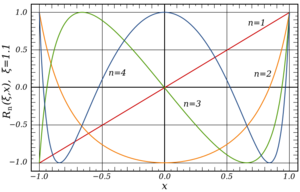
Plot of elliptic rational functions for x between -1 and 1 for orders 1,2,3 and 4 with discrimination factor ξ=1.1. All are bounded between -1 and 1 and all have the value 1 at x=1.

In mathematics the elliptic rational functions are a sequence of rational functions with real coefficients. Elliptic rational functions are extensively used in the design of elliptic electronic filters. (These functions are sometimes called Chebyshev rational functions, not to be confused with certain other functions of the same name).

Rational elliptic functions are identified by a positive integer order n and include a parameter ξ ≥ 1 called the selectivity factor. A rational elliptic function of degree n in x with selectivity factor ξ is generally defined as:

[math]\displaystyle{ R_n(\xi,x)\equiv \mathrm{cd}\left(n\frac{K(1/L_n(\xi))}{K(1/\xi)}\,\mathrm{cd}^{-1}(x,1/\xi),1/L_n(\xi)\right) }[/math]

where

  • cd(u,k) is the Jacobi elliptic cosine function.
  • K() is a complete elliptic integral of the first kind.
  • [math]\displaystyle{ L_n(\xi)=R_n(\xi,\xi) }[/math] is the discrimination factor, equal to the minimum value of the magnitude of [math]\displaystyle{ R_n(\xi,x) }[/math] for [math]\displaystyle{ |x|\ge\xi }[/math].

For many cases, in particular for orders of the form n = 2a3b where a and b are integers, the elliptic rational functions can be expressed using algebraic functions alone. Elliptic rational functions are closely related to the Chebyshev polynomials: Just as the circular trigonometric functions are special cases of the Jacobi elliptic functions, so the Chebyshev polynomials are special cases of the elliptic rational functions.

Expression as a ratio of polynomials

For even orders, the elliptic rational functions may be expressed as a ratio of two polynomials, both of order n.

[math]\displaystyle{ R_n(\xi,x)=r_0\,\frac{\prod_{i=1}^n (x-x_i)}{\prod_{i=1}^n (x-x_{pi})} }[/math]      (for n even)

where [math]\displaystyle{ x_i }[/math] are the zeroes and [math]\displaystyle{ x_{pi} }[/math] are the poles, and [math]\displaystyle{ r_0 }[/math] is a normalizing constant chosen such that [math]\displaystyle{ R_n(\xi,1)=1 }[/math]. The above form would be true for even orders as well except that for odd orders, there will be a pole at x=∞ and a zero at x=0 so that the above form must be modified to read:

[math]\displaystyle{ R_n(\xi,x)=r_0\,x\,\frac{\prod_{i=1}^{n-1} (x-x_i)}{\prod_{i=1}^{n-1} (x-x_{pi})} }[/math]      (for n odd)

Properties

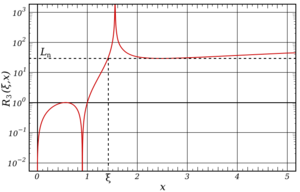
Plot of the absolute value of the third order elliptic rational function with ξ=1.4. There is a zero at x=0 and the pole at infinity. Since the function is antisymmetric, it is seen there are three zeroes and three poles. Between the zeroes, the function rises to a value of 1 and, between the poles, the function drops to the value of the discrimination factor Ln
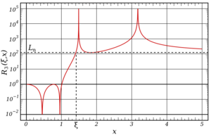
Plot of the absolute value of the fourth order elliptic rational function with ξ=1.4. Since the function is symmetric, it is seen that there are four zeroes and four poles. Between the zeroes, the function rises to a value of 1 and, between the poles, the function drops to the value of the discrimination factor Ln
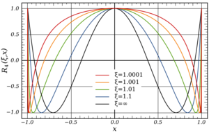
Plot of the effect of the selectivity factor ξ. The fourth order elliptic rational function is shown with values of ξ varying from nearly unity to infinity. The black curve, corresponding to ξ=∞ is the Chebyshev polynomial of order 4. The closer the selectivity factor is to unity, the steeper will be the slope in the transition region between x=1 and x=ξ.

The canonical properties

  • [math]\displaystyle{ R_n^2(\xi,x)\le 1 }[/math] for [math]\displaystyle{ |x|\le 1\, }[/math]
  • [math]\displaystyle{ R_n^2(\xi,x)= 1 }[/math] at [math]\displaystyle{ |x|= 1\, }[/math]
  • [math]\displaystyle{ R_n^2(\xi,-x)=R_n^2(\xi,x) }[/math]
  • [math]\displaystyle{ R_n^2(\xi,x)\gt 1 }[/math] for [math]\displaystyle{ x\gt 1\, }[/math]
  • The slope at x=1 is as large as possible
  • The slope at x=1 is larger than the corresponding slope of the Chebyshev polynomial of the same order.

The only rational function satisfying the above properties is the elliptic rational function (Lutovac Tošić). The following properties are derived:

Normalization

The elliptic rational function is normalized to unity at x=1:

[math]\displaystyle{ R_n(\xi,1)=1\, }[/math]

Nesting property

The nesting property is written:

[math]\displaystyle{ R_m(R_n(\xi,\xi),R_n(\xi,x))=R_{m\cdot n}(\xi,x)\, }[/math]

This is a very important property:

  • If [math]\displaystyle{ R_n }[/math] is known for all prime n, then nesting property gives [math]\displaystyle{ R_n }[/math] for all n. In particular, since [math]\displaystyle{ R_2 }[/math] and [math]\displaystyle{ R_3 }[/math] can be expressed in closed form without explicit use of the Jacobi elliptic functions, then all [math]\displaystyle{ R_n }[/math] for n of the form [math]\displaystyle{ n=2^a3^b }[/math] can be so expressed.
  • It follows that if the zeroes of [math]\displaystyle{ R_n }[/math] for prime n are known, the zeros of all [math]\displaystyle{ R_n }[/math] can be found. Using the inversion relationship (see below), the poles can also be found.
  • The nesting property implies the nesting property of the discrimination factor:
[math]\displaystyle{ L_{m\cdot n}(\xi)=L_m(L_n(\xi)) }[/math]

Limiting values

The elliptic rational functions are related to the Chebyshev polynomials of the first kind [math]\displaystyle{ T_n(x) }[/math] by:

[math]\displaystyle{ \lim_{\xi=\rightarrow\,\infty}R_n(\xi,x)=T_n(x)\, }[/math]

Symmetry

[math]\displaystyle{ R_n(\xi,-x)=R_n(\xi,x)\, }[/math] for n even
[math]\displaystyle{ R_n(\xi,-x)=-R_n(\xi,x)\, }[/math] for n odd

Equiripple

[math]\displaystyle{ R_n(\xi,x) }[/math] has equal ripple of [math]\displaystyle{ \pm 1 }[/math] in the interval [math]\displaystyle{ -1\le x\le 1 }[/math]. By the inversion relationship (see below), it follows that [math]\displaystyle{ 1/R_n(\xi,x) }[/math] has equiripple in [math]\displaystyle{ -1/\xi \le x\le 1/\xi }[/math] of [math]\displaystyle{ \pm 1/L_n(\xi) }[/math].

Inversion relationship

The following inversion relationship holds:

[math]\displaystyle{ R_n(\xi,\xi/x)=\frac{R_n(\xi,\xi)}{R_n(\xi,x)}\, }[/math]

This implies that poles and zeroes come in pairs such that

[math]\displaystyle{ x_{pi}x_{zi}=\xi\, }[/math]

Odd order functions will have a zero at x=0 and a corresponding pole at infinity.

Poles and Zeroes

The zeroes of the elliptic rational function of order n will be written [math]\displaystyle{ x_{ni}(\xi) }[/math] or [math]\displaystyle{ x_{ni} }[/math] when [math]\displaystyle{ \xi }[/math] is implicitly known. The zeroes of the elliptic rational function will be the zeroes of the polynomial in the numerator of the function.

The following derivation of the zeroes of the elliptic rational function is analogous to that of determining the zeroes of the Chebyshev polynomials (Lutovac Tošić). Using the fact that for any z

[math]\displaystyle{ \mathrm{cd}\left((2m-1)K\left(1/z\right),\frac{1}{z}\right)=0\, }[/math]

the defining equation for the elliptic rational functions implies that

[math]\displaystyle{ n \frac{K(1/L_n)}{K(1/\xi)}\mathrm{cd}^{-1}(x_m,1/\xi)=(2m-1)K(1/L_n) }[/math]

so that the zeroes are given by

[math]\displaystyle{ x_m=\mathrm{cd}\left(K(1/\xi)\,\frac{2m-1}{n},\frac{1}{\xi}\right). }[/math]

Using the inversion relationship, the poles may then be calculated.

From the nesting property, if the zeroes of [math]\displaystyle{ R_m }[/math] and [math]\displaystyle{ R_n }[/math] can be algebraically expressed (i.e. without the need for calculating the Jacobi ellipse functions) then the zeroes of [math]\displaystyle{ R_{m\cdot n} }[/math] can be algebraically expressed. In particular, the zeroes of elliptic rational functions of order [math]\displaystyle{ 2^i3^j }[/math] may be algebraically expressed (Lutovac Tošić). For example, we can find the zeroes of [math]\displaystyle{ R_8(\xi,x) }[/math] as follows: Define

[math]\displaystyle{ X_n\equiv R_n(\xi,x)\qquad L_n\equiv R_n(\xi,\xi)\qquad t_n\equiv \sqrt{1-1/L_n^2}. }[/math]

Then, from the nesting property and knowing that

[math]\displaystyle{ R_2(\xi,x)=\frac{(t+1)x^2-1}{(t-1)x^2+1} }[/math]

where [math]\displaystyle{ t\equiv \sqrt{1-1/\xi^2} }[/math] we have:

[math]\displaystyle{ L_2=\frac{1+t}{1-t},\qquad L_4=\frac{1+t_2}{1-t_2},\qquad L_8=\frac{1+t_4}{1-t_4} }[/math]
[math]\displaystyle{ X_2=\frac{(t+1)x^2 -1}{(t-1)x^2 +1},\qquad X_4=\frac{(t_2+1)X_2^2-1}{(t_2-1)X_2^2+1},\qquad X_8=\frac{(t_4+1)X_4^2-1}{(t_4-1)X_4^2+1}. }[/math]

These last three equations may be inverted:

[math]\displaystyle{ x =\frac{1}{\pm\sqrt{1+t \,\left(\frac{1-X_2}{1+X_2}\right)}},\qquad X_2=\frac{1}{\pm\sqrt{1+t_2\,\left(\frac{1-X_4}{1+X_4}\right)}},\qquad X_4=\frac{1}{\pm\sqrt{1+t_4\,\left(\frac{1-X_8}{1+X_8}\right)}}.\qquad }[/math]

To calculate the zeroes of [math]\displaystyle{ R_8(\xi,x) }[/math] we set [math]\displaystyle{ X_8=0 }[/math] in the third equation, calculate the two values of [math]\displaystyle{ X_4 }[/math], then use these values of [math]\displaystyle{ X_4 }[/math] in the second equation to calculate four values of [math]\displaystyle{ X_2 }[/math] and finally, use these values in the first equation to calculate the eight zeroes of [math]\displaystyle{ R_8(\xi,x) }[/math]. (The [math]\displaystyle{ t_n }[/math] are calculated by a similar recursion.) Again, using the inversion relationship, these zeroes can be used to calculate the poles.

Particular values

We may write the first few elliptic rational functions as:

[math]\displaystyle{ R_1(\xi,x)=x\, }[/math]
[math]\displaystyle{ R_2(\xi,x)=\frac{(t+1)x^2-1}{(t-1)x^2+1} }[/math]
where
[math]\displaystyle{ t \equiv \sqrt{1-\frac{1}{\xi^2}} }[/math]
[math]\displaystyle{ R_3(\xi,x)=x\,\frac{(1-x_p^2)(x^2-x_z^2)}{(1-x_z^2)(x^2-x_p^2)} }[/math]
where
[math]\displaystyle{ G\equiv\sqrt{4\xi^2+(4\xi^2(\xi^2\!-\!1))^{2/3}} }[/math]
[math]\displaystyle{ x_p^2\equiv\frac{2\xi^2\sqrt{G}}{\sqrt{8\xi^2(\xi^2\!+\!1)+12G\xi^2-G^3}-\sqrt{G^3}} }[/math]
[math]\displaystyle{ x_z^2=\xi^2/x_p^2 }[/math]
[math]\displaystyle{ R_4(\xi,x)=R_2(R_2(\xi,\xi),R_2(\xi,x))=\frac {(1+t)(1+\sqrt{t})^2x^4-2(1+t)(1+\sqrt{t})x^2+1} {(1+t)(1-\sqrt{t})^2x^4-2(1+t)(1-\sqrt{t})x^2+1} }[/math]
[math]\displaystyle{ R_6(\xi,x)=R_3(R_2(\xi,\xi),R_2(\xi,x))\, }[/math] etc.

See (Lutovac Tošić) for further explicit expressions of order n=5 and [math]\displaystyle{ n=2^i\,3^j }[/math].

The corresponding discrimination factors are:

[math]\displaystyle{ L_1(\xi)=\xi\, }[/math]
[math]\displaystyle{ L_2(\xi)=\frac{1+t}{1-t}=\left(\xi+\sqrt{\xi^2-1}\right)^2 }[/math]
[math]\displaystyle{ L_3(\xi)=\xi^3\left(\frac{1-x_p^2}{\xi^2-x_p^2}\right)^2 }[/math]
[math]\displaystyle{ L_4(\xi)=\left(\sqrt{\xi}+(\xi^2-1)^{1/4}\right)^4\left(\xi+\sqrt{\xi^2-1}\right)^2 }[/math]
[math]\displaystyle{ L_6(\xi)=L_3(L_2(\xi))\, }[/math] etc.

The corresponding zeroes are [math]\displaystyle{ x_{nj} }[/math] where n is the order and j is the number of the zero. There will be a total of n zeroes for each order.

[math]\displaystyle{ x_{11}=0\, }[/math]
[math]\displaystyle{ x_{21}=\xi\sqrt{1-t}\, }[/math]
[math]\displaystyle{ x_{22}=-x_{21}\, }[/math]
[math]\displaystyle{ x_{31}=x_z\, }[/math]
[math]\displaystyle{ x_{32}=0\, }[/math]
[math]\displaystyle{ x_{33}=-x_{31}\, }[/math]
[math]\displaystyle{ x_{41}=\xi\sqrt{\left(1-\sqrt{t}\right)\left(1+t-\sqrt{t(t+1)}\right)}\, }[/math]
[math]\displaystyle{ x_{42}=\xi\sqrt{\left(1-\sqrt{t}\right)\left(1+t+\sqrt{t(t+1)}\right)}\, }[/math]
[math]\displaystyle{ x_{43}=-x_{42}\, }[/math]
[math]\displaystyle{ x_{44}=-x_{41}\, }[/math]

From the inversion relationship, the corresponding poles [math]\displaystyle{ x_{p,ni} }[/math] may be found by [math]\displaystyle{ x_{p,ni}=\xi/(x_{ni}) }[/math]

References

  • MathWorld
  • Daniels, Richard W. (1974). Approximation Methods for Electronic Filter Design. New York: McGraw-Hill. ISBN 0-07-015308-6. 
  • Lutovac, Miroslav D.; Tošić, Dejan V.; Evans, Brian L. (2001). Filter Design for Signal Processing using MATLAB© and Mathematica©. New Jersey, USA: Prentice Hall. ISBN 0-201-36130-2.