Finance:Marginal revenue

Marginal revenue (or marginal benefit) is a central concept in microeconomics that describes the additional total revenue generated by increasing product sales by 1 unit.[1][2][3][4][5] Marginal revenue is the increase in revenue from the sale of one additional unit of product, i.e., the revenue from the sale of the last unit of product. It can be positive or negative. Marginal revenue is an important concept in vendor analysis.[6][7] To derive the value of marginal revenue, it is required to examine the difference between the aggregate benefits a firm received from the quantity of a good and service produced last period and the current period with one extra unit increase in the rate of production.[8] Marginal revenue is a fundamental tool for economic decision making within a firm's setting, together with marginal cost to be considered.[9]
In a perfectly competitive market, the incremental revenue generated by selling an additional unit of a good is equal to the price the firm is able to charge the buyer of the good.[3][10] This is because a firm in a competitive market will always get the same price for every unit it sells regardless of the number of units the firm sells since the firm's sales can never impact the industry's price.[1][3] Therefore, in a perfectly competitive market, firms set the price level equal to their marginal revenue .[8]
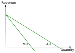
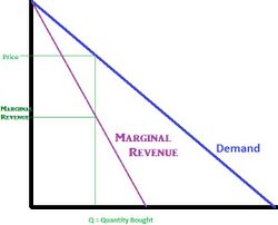
In imperfect competition, a monopoly firm is a large producer in the market and changes in its output levels impact market prices, determining the whole industry's sales. Therefore, a monopoly firm lowers its price on all units sold in order to increase output (quantity) by 1 unit.[1][3][8] Since a reduction in price leads to a decline in revenue on each good sold by the firm, the marginal revenue generated is always lower than the price level charged .[1][3][8] The marginal revenue (the increase in total revenue) is the price the firm gets on the additional unit sold, less the revenue lost by reducing the price on all other units that were sold prior to the decrease in price. Marginal revenue is the concept of a firm sacrificing the opportunity to sell the current output at a certain price, in order to sell a higher quantity at a reduced price.[8]
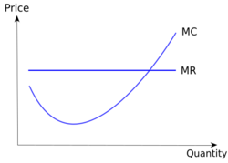
Profit maximization occurs at the point where marginal revenue (MR) equals marginal cost (MC). If then a profit-maximizing firm will increase output to generate more profit, while if then the firm will decrease output to gain additional profit. Thus the firm will choose the profit-maximizing level of output for which .[11]
Definition
Marginal revenue is equal to the ratio of the change in revenue for some change in quantity sold to that change in quantity sold. This can be formulated as:[12]
This can also be represented as a derivative when the change in quantity sold becomes arbitrarily small. Define the revenue function to be[13]
where Q is output and P(Q) is the inverse demand function of customers. By the product rule, marginal revenue is then given by
where the prime sign indicates a derivative. For a firm facing perfect competition, price does not change with quantity sold (), so marginal revenue is equal to price. For a monopoly, the price decreases with quantity sold (), so marginal revenue is less than price for positive (see Example 1).[8]
Example 1: If a firm sells 20 units of books (quantity) for $50 each (price), this earns total revenue: P*Q = $50*20 = $1000
Then if the firm increases quantity sold to 21 units of books at $49 each, this earns total revenue: P*Q = $49*21 = $1029
Therefore, using the marginal revenue formula (MR)[12] =
Example 2: If a firm's total revenue function is written as [14]
Then, by first order derivation, marginal revenue would be expressed as
Therefore, if Q = 40,
MR = 200 − 2(40) = $120
Marginal revenue curve


The marginal revenue curve is affected by the same factors as the demand curve – changes in income, changes in the prices of complements and substitutes, changes in populations, etc.[15] These factors can cause the MR curve to shift and rotate.[16] Marginal revenue curve differs under perfect competition and imperfect competition (monopoly).[17]
Under perfect competition, there are multiple firms present in the market. Changes in the supply level of a single firm does not have an impact on the total price in the market.[18] Firms follow the price determined by market equilibrium of supply and demand and are price takers.[19] The marginal revenue curve is a horizontal line at the market price, implying perfectly elastic demand and is equal to the demand curve.[20]
Under monopoly, one firm is a sole seller in the market with a differentiated product.[17] The supply level (output) and price is determined by the monopolist in order to maximise profits, making a monopolist a price maker.[21] The marginal revenue for a monopolist is the private gain of selling an additional unit of output. The marginal revenue curve is downward sloping and below the demand curve and the additional gain from increasing the quantity sold is lower than the chosen market price.[22][23] Under monopoly, the price of all units lowers each time a firm increases its output sold, this causes the firm to face a diminishing marginal revenue.[24]
Marginal revenue curve and marginal cost curve
A company will stop producing a product/service when marginal revenue (money the company earns from each additional sale) equals marginal cost (the cost the company costs to produce an additional unit). Therefore, a company is making money when MR is greater than marginal cost (MC). And when MC = MR, it is called profit maximization. After this point; the company can no longer make a profit. Therefore, it is in their interest to stop production.[25]
Relationship between marginal revenue and elasticity
The relationship between marginal revenue and the elasticity of demand by the firm's customers can be derived as follows:[26][27][28]
- Taking the first order derivative of total revenue:
where R is total revenue, P(Q) is the inverse of the demand function, and e < 0 is the price elasticity of demand written as .[27]
Monopolist firm, as a price maker in the market, has the incentives to lower prices to boost quantities sold.[17] The price effects occur when a firm raises its products' prices and increased revenue on each unit sold. The quantity effect, on the other hand, describes the stage when prices increased and consumers quantity demanded reduce. Firms' pricing decision, therefore, is based on the tradeoff between the two outcomes by considering elasticity.[29]
When a monopolist firm is facing an Inelastic demand curve (e<1), it implies that a percentage change in quantity is less than the percentage change in price. By increasing quantity sold, the firm is forced to accept a reduction of price for all the current and previous production units,[23] resulting in a negative marginal revenue (MR). As such, as consumers are less sensitive and responsive to lower prices movement and so the expected product sales boost is highly unlikely and firms lose more profits due to reduction in marginal revenue. A rational firm will have to maintain its current price levels instead or increase the price for profit expansion.[27][30][31]
Increases in consumer's responsiveness to small changes in prices leads represents an elastic demand curve (e>1), resulting in a positive marginal revenue (MR) under monopoly competition. This signifies that a percentage change in quantity outweighs the percentage change in price. Firms in the imperfect competition market that lower prices by a small portion benefit from a large percentage increase in quantity sold and this generates greater marginal revenue. With that, a rational firm will recognize the value of price effects under an elastic demand function for its products and would avoid increasing prices as the quantity (demand) lost would be amplified due to the elastic demand curve.[27][30][31]
If the firm is a perfect competitor, where quantity produced and sold has no effect on the market price, then the price elasticity of demand is negative infinity and marginal revenue simply equals the (market-determined) price .[27][31]
Therefore, it is essential to be aware of the elasticity of demand. A monopolist prefers to be on the more elastic end of the demand curve in order to gain a positive marginal revenue. This shows that a monopolist reduces output produced up to the point where marginal revenue is positive.[27][28]
Marginal revenue and Marginal benefit
Example 1: Suppose consumers want to buy an additional lipstick. If the consumer is willing to pay $50 for this extra lipstick, the marginal income of the purchase is $50. However, the more lipsticks consumers have, the less they pay for the next lipstick. This is because as consumers accumulate more and more lipsticks, the benefits of having an additional lipstick will be reduced.
Example 2: Suppose customers are considering buying 10 computers. If the marginal income of the 11th computer is $2, and the computer company is willing to sell the 11th component to maximize its consumer interest, the company's marginal income is $2 and consumers' marginal income is $2.
law of diminishing marginal returns
In microeconomics, for every unit of input added to a firm, the return received decreases. When a variable factor of production is put into a firm at a constant level of technology, the initial increase in this factor of production will increase output, but when it exceeds a certain limit, the increased output will diminish and will eventually reduce output in absolute terms.[32]
law of increasing marginal returns
In contrast to the law of diminishing marginal returns, in a knowledge-dependent economy, as knowledge and technological inputs increase, the output increases and the producer's returns tend to increase. This is an example of increasing marginal revenue; suppose a company produces toy airplanes. After some production, the company spends $10 in materials and labor to build the 1st toy airplane. The 1st toy airplane sells for $15, which means the profit on that toy is $5. Now, suppose that the 2nd toy airplane also costs $10, but this time it can be sold for $17. The profit on the 2nd toy airplane is $12 greater than the profit on the 1st toy airplane.
Marginal revenue and markup pricing
Profit maximization requires that a firm produces where marginal revenue equals marginal costs. Firm managers are unlikely to have complete information concerning their marginal revenue function or their marginal costs. However, the profit maximization conditions can be expressed in a “more easily applicable form”:
- MR = MC,
- MR = P(1 + 1/e),
- MC = P(1 + 1/e),
- MC = P + P/e,
- (P − MC)/ P = −1/e.[33]
Markup is the difference between price and marginal cost. The formula states that markup as a percentage of price equals the negative (and hence the absolute value) of the inverse of the elasticity of demand.[33] A lower elasticity of demand implies a higher markup at the profit maximising equilibrium.[31]
(P − MC)/ P = −1/e is called the Lerner index after economist Abba Lerner.[34] The Lerner index is a measure of market power — the ability of a firm to charge a price that exceeds marginal cost. The index varies from zero (when demand is infinitely elastic (a perfectly competitive market) to 1 (when demand has an elasticity of −1). The closer the index value is to 1, the greater is the difference between price and marginal cost. The Lerner index increases as demand becomes less elastic.[34]
Alternatively, the relationship can be expressed as:
- P = MC/(1 + 1/e).
Thus, for example, if e is −2 and MC is $5.00 then price is $10.00.
Example If a company can sell 10 units at $20 each or 11 units at $19 each, then the marginal revenue from the eleventh unit is (11 × 19) − (10 × 20) = $9.
See also
Notes
- ↑ 1.0 1.1 1.2 1.3 Bradley R. chiller, "Essentials of Economics", New York: McGraw-Hill, Inc., 1991.
- ↑ Edwin Mansfield, "Micro-Economics Theory and Applications, 3rd Edition", New York and London:W.W. Norton and Company, 1979.
- ↑ 3.0 3.1 3.2 3.3 3.4 Roger LeRoy Miller, "Intermediate Microeconomics Theory Issues Applications, Third Edition", New York: McGraw-Hill, Inc, 1982.
- ↑ Tirole, Jean, "The Theory of Industrial Organization", Cambridge, Massachusetts: The MIT Press, 1988.
- ↑ John Black, "Oxford Dictionary of Economics", New York: Oxford University Press, 2003.
- ↑ Primont, D. F., & Primont, D. (1995). Further Evidence of Positively Sloping Marginal Revenue. Southern Economic Journal, 62(2), 481–485. https://doi.org/10.2307/1060699
- ↑ Wilson, T. (1979). The Price of Oil: A Case of Negative Marginal Revenue. The Journal of Industrial Economics, 27(4), 301–315. https://doi.org/10.2307/2097955
- ↑ 8.0 8.1 8.2 8.3 8.4 8.5 Schiller, Bradley R.; Gebhardt, Karen (2017). Essentials of economics (10th ed.). New York: McGraw-Hill/Irwin. ISBN 978-1-259-23570-2. OCLC 955345952.
- ↑ Mankiw, N. Gregory (2009). Principles of microeconomics (5th ed.). Mason, OH: South-Western Cengage Learning. ISBN 978-0-324-58998-6. OCLC 226358094.
- ↑ O'Sullivan & Sheffrin (2003), p. 112.
- ↑ Fisher, Timothy C. G.; Prentice, David; Waschik, Robert G. (2010). Managerial economics : a strategic approach. Routledge. p. 33. ISBN 9780415495172. OCLC 432989728.
- ↑ 12.0 12.1 Pindyck, Robert S. (3 December 2014). Microeconomics. Rubinfeld, Daniel L. (Global edition, Eighth ed.). Boston [Massachusetts]. ISBN 978-1-292-08197-7. OCLC 908406121. https://www.worldcat.org/oclc/908406121.
- ↑ "3.2: Monopoly Profit-Maximizing Solution" (in en). 2020-02-27. https://socialsci.libretexts.org/Bookshelves/Economics/Book%3A_The_Economics_of_Food_and_Agricultural_Markets_(Barkley)/03%3A_Monopoly_and_Market_Power/3.02%3A_Monopoly_Profit-Maximizing_Solution.
- ↑ Goldstein, Larry Joel; Lay, David C.; Schneider, David I. (2004). Brief calculus & its applications (10th ed.). Upper Saddle River, NJ: Pearson Education. ISBN 0-13-046618-2. OCLC 50235091.
- ↑ Landsburg, Steven E. (2013). Price theory and applications (Ninth ed.). Stamford, CT. ISBN 978-1-285-42352-4. OCLC 891601555.
- ↑ Landsburg, S Price 2002. p. 137.
- ↑ 17.0 17.1 17.2 Kumar, Manoj (2015-05-08). "Revenue Curves under Different Markets (With Diagram)" (in en-US). https://www.economicsdiscussion.net/revenue/revenue-curves-under-different-markets-with-diagram/6877.
- ↑ "The Supply Curve of a Competitive Firm". https://saylordotorg.github.io/text_microeconomics-theory-through-applications/s10-05-the-supply-curve-of-a-competit.html.
- ↑ "Demand in a Perfectly Competitive Market". https://www.cliffsnotes.com/study-guides/economics/perfect-competition/demand-in-a-perfectly-competitive-market.
- ↑ Russell W. Cooper; Alun Andrew John (2011). Microeconomics : theory through applications. Arlington, Virginia. ISBN 978-1-4533-1328-2. OCLC 953968136.
- ↑ McLean, William J. (William Joseph) (2013). Economics and contemporary issues. Applegate, Michael. (9e ed.). Mason, Ohio: South-Western Cengage Learning. ISBN 978-1-111-82339-9. OCLC 775406167. https://www.worldcat.org/oclc/775406167.
- ↑ Tuovila, Alicia. "Marginal Revenue (MR) Definition" (in en). https://www.investopedia.com/terms/m/marginal-revenue-mr.asp.
- ↑ 23.0 23.1 "Marginal revenue for a monopolist". https://www.economics.utoronto.ca/osborne/2x3/tutorial/MR.HTM.
- ↑ "The Monopoly Model". https://saylordotorg.github.io/text_principles-of-microeconomics-v2.0/s13-02-the-monopoly-model.html.
- ↑ Boyce, Paul (February 6, 2021). "Marginal Revenue Definition". https://boycewire.com/marginal-revenue-definition/.
- ↑ Perloff (2008) p. 364.
- ↑ 27.0 27.1 27.2 27.3 27.4 27.5 "3.3: Marginal Revenue and the Elasticity of Demand" (in en). 2020-02-27. https://socialsci.libretexts.org/Bookshelves/Economics/Book%3A_The_Economics_of_Food_and_Agricultural_Markets_(Barkley)/03%3A_Monopoly_and_Market_Power/3.03%3A_Marginal_Revenue_and_the_Elasticity_of_Demand.
- ↑ 28.0 28.1 Rekhi, Samia (2016-05-16). "Marginal Revenue and Price Elasticity of Demand" (in en-US). https://www.economicsdiscussion.net/price-elasticity/marginal-revenue-and-price-elasticity-of-demand/19728.
- ↑ Paul Krugman; Robin Wells; Iris Au; Jack Parkinson (2013). Microeconomics (3rd ed.). New York: Worth Publishers. ISBN 978-1-4292-4005-5. OCLC 796082268.
- ↑ 30.0 30.1 Pemberton, Malcolm; Rau, Nicholas (2011). Mathematics for economists : an introductory textbook (3rd ed.). Manchester: Manchester University Press. ISBN 978-0-7190-8705-9. OCLC 756276243.
- ↑ 31.0 31.1 31.2 31.3 "Leibniz: The elasticity of demand" (in en). http://www.core-econ.org/the-economy/book/text/leibniz-07-08-01.html.
- ↑ Bondarenko, Peter. "microeconomics". Encyclopedia Britannica, Mar 25, 2023, https://www.britannica.com/topic/microeconomics. Accessed 21 April 2023.
- ↑ 33.0 33.1 Pindyck, R & Rubinfeld, D (2001) p. 334.
- ↑ 34.0 34.1 Perloff (2008) p. 371.
References
- Landsburg, S 2002 Price Theory & Applications, 5th ed. South-Western.
- Perloff, J., 2008, Microeconomics: Theory & Applications with Calculus, Pearson. ISBN 9780321277947
- Pindyck, R & Rubinfeld, D 2001: Microeconomics 5th ed. Page Prentice-Hall. ISBN 0-13-019673-8
- Samuelson & Marks, 2003 Managerial Economics 4th ed. Wiley
- O'Sullivan, Arthur; Sheffrin, Steven M. (2003). Economics: Principles in Action. Pearson Prentice Hall. ISBN 0-13-063085-3.
 |
