Gradient vector flow
Gradient vector flow (GVF), a computer vision framework introduced by Chenyang Xu and Jerry L. Prince,[1][2] is the vector field that is produced by a process that smooths and diffuses an input vector field. It is usually used to create a vector field from images that points to object edges from a distance. It is widely used in image analysis and computer vision applications for object tracking, shape recognition, segmentation, and edge detection. In particular, it is commonly used in conjunction with active contour model.

Background
Finding objects or homogeneous regions in images is a process known as image segmentation. In many applications, the locations of object edges can be estimated using local operators that yield a new image called an edge map. The edge map can then be used to guide a deformable model, sometimes called an active contour or a snake, so that it passes through the edge map in a smooth way, therefore defining the object itself.
A common way to encourage a deformable model to move toward the edge map is to take the spatial gradient of the edge map, yielding a vector field. Since the edge map has its highest intensities directly on the edge and drops to zero away from the edge, these gradient vectors provide directions for the active contour to move. When the gradient vectors are zero, the active contour will not move, and this is the correct behavior when the contour rests on the peak of the edge map itself. However, because the edge itself is defined by local operators, these gradient vectors will also be zero far away from the edge and therefore the active contour will not move toward the edge when initialized far away from the edge.
Gradient vector flow (GVF) is the process that spatially extends the edge map gradient vectors, yielding a new vector field that contains information about the location of object edges throughout the entire image domain. GVF is defined as a diffusion process operating on the components of the input vector field. It is designed to balance the fidelity of the original vector field, so it is not changed too much, with a regularization that is intended to produce a smooth field on its output.
Although GVF was designed originally for the purpose of segmenting objects using active contours attracted to edges, it has been since adapted and used for many alternative purposes. Some newer purposes including defining a continuous medial axis representation,[3] regularizing image anisotropic diffusion algorithms,[4] finding the centers of ribbon-like objects,[5] constructing graphs for optimal surface segmentations,[6] creating a shape prior,[7] and much more.
Theory
The theory of GVF was originally described by Xu and Prince.[2] Let be an edge map defined on the image domain. For uniformity of results, it is important to restrict the edge map intensities to lie between 0 and 1, and by convention takes on larger values (close to 1) on the object edges. The gradient vector flow (GVF) field is given by the vector field that minimizes the energy functional
|
|
( 1 ) |
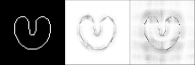
In this equation, subscripts denote partial derivatives and the gradient of the edge map is given by the vector field . Figure 1 shows an edge map, the gradient of the (slightly blurred) edge map, and the GVF field generated by minimizing .

Equation 1 is a variational formulation that has both a data term and a regularization term. The first term in the integrand is the data term. It encourages the solution to closely agree with the gradients of the edge map since that will make small. However, this only needs to happen when the edge map gradients are large since is multiplied by the square of the length of these gradients. The second term in the integrand is a regularization term. It encourages the spatial variations in the components of the solution to be small by penalizing the sum of all the partial derivatives of . As is customary in these types of variational formulations, there is a regularization parameter that must be specified by the user in order to trade off the influence of each of the two terms. If is large, for example, then the resulting field will be very smooth and may not agree as well with the underlying edge gradients.
Theoretical Solution. Finding to minimize Equation 1 requires the use of calculus of variations since is a function, not a variable. Accordingly, the Euler equations, which provide the necessary conditions for to be a solution can be found by calculus of variations, yielding
-
( 2a)
-
( 2b)
where is the Laplacian operator. It is instructive to examine the form of the equations in (2). Each is a partial differential equation that the components and of must satisfy. If the magnitude of the edge gradient is small, then the solution of each equation is guided entirely by Laplace's equation, for example , which will produce a smooth scalar field entirely dependent on its boundary conditions. The boundary conditions are effectively provided by the locations in the image where the magnitude of the edge gradient is large, where the solution is driven to agree more with the edge gradients.
Computational Solutions. There are two fundamental ways to compute GVF. First, the energy function itself (1) can be directly discretized and minimized, for example, by gradient descent. Second, the partial differential equations in (2) can be discretized and solved iteratively. The original GVF paper used an iterative approach, while later papers introduced considerably faster implementations such as an octree-based method,[8] a multi-grid method,[9] and an augmented Lagrangian method.[10] In addition, very fast GPU implementations have been developed in[11][12]
Extensions and Advances. GVF is easily extended to higher dimensions. The energy function is readily written in a vector form as
|
|
( 3 ) |
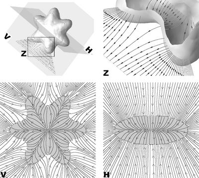
which can be solved by gradient descent or by finding and solving its Euler equation. Figure 2 shows an illustration of a three-dimensional GVF field on the edge map of a simple object (see [13]).

The data and regularization terms in the integrand of the GVF functional can also be modified. A modification described in ,[14] called generalized gradient vector flow (GGVF) defines two scalar functions and reformulates the energy as
|
|
( 4 ) |
While the choices and reduce GGVF to GVF, the alternative choices and , for a user-selected constant, can improve the tradeoff between the data term and its regularization in some applications.
The GVF formulation has been further extended to vector-valued images in [15] where a weighted structure tensor of a vector-valued image is used. A learning based probabilistic weighted GVF extension was proposed in [16] to further improve the segmentation for images with severely cluttered textures or high levels of noise.
The variational formulation of GVF has also been modified in motion GVF (MGVF) to incorporate object motion in an image sequence.[17] Whereas the diffusion of GVF vectors from a conventional edge map acts in an isotropic manner, the formulation of MGVF incorporates the expected object motion between image frames.
An alternative to GVF called vector field convolution (VFC) provides many of the advantages of GVF, has superior noise robustness, and can be computed very fast.[18] The VFC field is defined as the convolution of the edge map with a vector field kernel
|
|
( 5 ) |
where
|
|
( 6 ) |
The vector field kernel has vectors that always point toward the origin but their magnitudes, determined in detail by the function , decrease to zero with increasing distance from the origin.
The beauty of VFC is that it can be computed very rapidly using a fast Fourier transform (FFT), a multiplication, and an inverse FFT. The capture range can be large and is explicitly given by the radius of the vector field kernel. A possible drawback of VFC is that weak edges might be overwhelmed by strong edges, but that problem can be alleviated by the use of a hybrid method that switches to conventional forces when the snake gets close to the boundary.
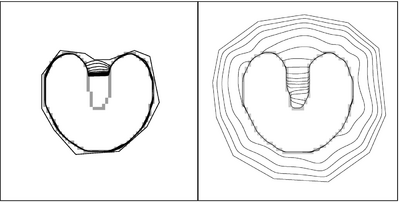
Properties. GVF has characteristics that have made it useful in many diverse applications. It has already been noted that its primary original purpose was to extend a local edge field throughout the image domain, far away from the actual edge in many cases. This property has been described as an extension of the capture range of the external force of an active contour model. It is also capable of moving active contours into concave regions of an object's boundary. These two properties are illustrated in Figure 3.

Previous forces that had been used as external forces (based on the edge map gradients and simply related variants) required pressure forces in order to move boundaries from large distances and into concave regions. Pressure forces, also called balloon forces, provide continuous force on the boundary in one direction (outward or inward), and tend to have the effect of pushing through weak boundaries. GVF can often replace pressure forces and yield better performance in such situations.
Because the diffusion process is inherent in the GVF solution, vectors that point in opposite directions tend to compete as they meet at a central location, thereby defining a type of geometric feature that is related to the boundary configuration, but not directly evident from the edge map. For example, perceptual edges are gaps in the edge map which tend to be connected visually by human perception.[19] GVF helps to connect them by diffusing opposing edge gradient vectors across the gap; and even though there is no actual edge map, active contour will converge to the perceptual edge because the GVF vectors drive them there (see Xu, C.; Prince, J.L. (2012). "Active contours, deformable models, and gradient vector flow". Online resource including code download. http://www.iacl.ece.jhu.edu/static/gvf.). This property carries over when there are so-called weak edges identified by regions of edge maps having lower values.
GVF vectors also meet in opposition at central locations of objects thereby defining a type of medialness. This property has been exploited as an alternative definition of the skeleton of objects[20] and also as a way to initialize deformable models within objects such that convergence to the boundary is more likely.
Applications
The most fundamental application of GVF is as an external force in a deformable model. A typical application considers an image with an object delineated by intensity from its background. Thus, a suitable edge map could be defined by
|
|
( 7 ) |
where is a Gaussian blurring kernel with standard deviation and is convolution. This definition is applicable in any dimension and yields an edge map that falls in the range . Gaussian blurring is used primarily so that a meaningful gradient vector can always be computed, but is generally kept fairly small so that true edge positions are not overly distorted. Given this edge map, the GVF vector field can be computed by solving (2).
The deformable model itself can be implemented in a variety of ways including parametric models such as the original snake[19] or active surfaces and implicit models including geometric deformable models.[21] In the case of parametric deformable models, the GVF vector field can be used directly as the external forces in the model. If the deformable model is defined by the evolution of the (two-dimensional) active contour , then a simple parametric active contour evolution equation can be written as
|
|
( 8 ) |
Here, the subscripts indicate partial derivatives and and are user-selected constants.

In the case of geometric deformable models, then the GVF vector field is first projected against the normal direction of the implicit wavefront, which defines an additional speed function. Accordingly, then the evolution of the signed distance function defining a simple geometric deformable contour can be written as
|
|
( 9 ) |
where is the curvature of the contour and is a user-selected constant.
A more sophisticated deformable model formulation that combines the geodesic active contour flow with GVF forces was proposed in .[22] This paper also shows how to apply the Additive Operator Splitting schema[23] for rapid computation of this segmentation method. The uniqueness and existence of this combined model were proven in .[24] A further modification of this model by using an external force term minimizing GVF divergence was proposed in [25] to achieve even better segmentation for images with complex geometric objects.
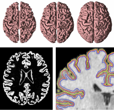
GVF has been used to find both inner, central, and central cortical surfaces in the analysis of brain images,[5] as shown in Figure 4. The process first finds the inner surface using a three-dimensional geometric deformable model with conventional forces. Then the central surface is found by exploiting the central tendency property of GVF. In particular, the cortical membership function of the human brain cortex, derived using a fuzzy classifier, is used to compute GVF as if itself were a thick edge map. The computed GVF vectors point towards the center of the cortex and can then be used as external forces to drive the inner surface to the central surface. Finally, another geometric deformable model with conventional forces is used to drive the central surface to a position on the outer surface of the cortex.
Several notable recent applications of GVF include constructing graphs for optimal surface segmentation in spectral-domain optical coherence tomography volumes,[6] a learning based probabilistic GVF active contour formulation to give more weights to objects of interest in ultrasound image segmentation,[16] and an adaptive multi-feature GVF active contour for improved ultrasound image segmentation without hand-tuned parameters.[26]
Related concepts
References
- ↑ Xu, C.; Prince, J.L. (June 1997). "Gradient Vector Flow: A New External Force for Snakes". Los Alamitos: Comp. Soc. Press. pp. 66–71. http://iacl.ece.jhu.edu/pubs/p087c.pdf.
- ↑ 2.0 2.1 Xu, C.; Prince, J.L. (1998). "Snakes, Shapes, and Gradient Vector Flow". IEEE Transactions on Image Processing 7 (3): 359–369. http://iacl.ece.jhu.edu/pubs/p084j.pdf.
- ↑ Hassouna, M.S.; Farag, A.Y. (2009). "Variational curve skeletons using gradient vector flow". IEEE Transactions on Pattern Analysis and Machine Intelligence 31 (12): 2257–2274.
- ↑ Yu, H.; Chua, C.S. (2006). "GVF-based anisotropic diffusion models". IEEE Transactions on Image Processing 15 (6): 1517–1524.
- ↑ 5.0 5.1 Han, X.Expression error: Unrecognized word "etal". (2004). "CRUISE: cortical reconstruction using implicit surface evolution". NeuroImage 23 (3): 997–1012.
- ↑ 6.0 6.1 Miri, M.S.; Robles, V.A.; Abràmoff, M.D.; Kwon, Y.H.; Garvin, M.K. (2017). "Incorporation of gradient vector flow field in a multimodal graph-theoretic approach for segmenting the internal limiting membrane from glaucomatous optic nerve head-centered SD-OCT volumes". Computerized Medical Imaging and Graphics 55: 87–94.
- ↑ Bai, J.; Shah, A.; Wu, X. (2018). "Optimal multi-object segmentation with novel gradient vector flow based shape priors". Computerized Medical Imaging and Graphics (Elsevier) 69: 96–111.
- ↑ Esteban, C. H.; Schmitt, F. (2004). "Silhouette and stereo fusion for 3D object modeling". Computer Vision and Image Understanding (Elsevier) 96 (3): 367–392.
- ↑ Han, X.; Xu, C.; Prince, J.L. (2007). "Fast numerical scheme for gradient vector flow computation using a multigrid method". IET Image Processing 1 (1): 48–55.
- ↑ Ren, D.; Zuo, W.; Zhao, X.; Lin, Z.; Zhang, D. (2013). "Fast gradient vector flow computation based on augmented Lagrangian method". Pattern Recognition Letters (Elsevier) 34 (2): 219–225.
- ↑ Smistad, E.; Elster, A.C.; Lindseth, F. (2015). "Real-time gradient vector flow on GPUs using OpenCL". Journal of Real-Time Image Processing (Springer) 10 (1): 67–74.
- ↑ Smistad, E.; Lindseth, F. (2016). "Multigrid gradient vector flow computation on the GPU". Journal of Real-Time Image Processing (Springer) 12 (3): 593–601.
- ↑ Xu, C.; Han, X.; Prince, J.L. (2008). "Gradient Vector Flow Deformable Models". in Isaac Bankman. Handbook of Medical Image Processing and Analysis (2nd ed.). Academic Press. pp. 181–194.
- ↑ Xu, C.; Prince, J.L. (1998). "Generalized gradient vector flow external forces for active contours". Signal Processing 71 (2): 131–139.
- ↑ Jaouen, V.Expression error: Unrecognized word "etal". (2014). "Variational segmentation of vector-valued images with gradient vector flow". IEEE Transactions on Image Processing 23 (11): 4773–4785.
- ↑ 16.0 16.1 Hafiane, A.; Vieyres, P.; Delbos, A. (2014). "Phase-based probabilistic active contour for nerve detection in ultrasound images for regional anesthesia". Computers in Biology and Medicine 52: 88–95.
- ↑ Ray, N.; Acton, S.T. (2004). "Motion gradient vector flow: An external force for tracking rolling leukocytes with shape and size constrained active contours". IEEE Transactions on Medical Imaging 23 (12): 1466–1478.
- ↑ Li, B.; Acton, S.T. (2007). "Active contour external force using vector field convolution for image segmentation". IEEE Transactions on Image Processing 16 (8): 2096–2106.
- ↑ 19.0 19.1 Kass, M.; Witkin, A.; Terzopoulos, D. (1988). "Snakes: active contour models". International Journal of Computer Vision 1: 321–331.
- ↑ Hassouna, M.S.; Farag, A.Y. (2009). "Variational curve skeletons using gradient vector flow". IEEE Transactions on Pattern Analysis and Machine Intelligence 31 (12): 2257–2274.
- ↑ Xu, C.; Yezzi, A.; Prince, J.L. (October 2000). "On the relationship between parametric and geometric active contours and its applications". 1. pp. 483–489.
- ↑ Paragios, N.; Mellina-Gottardo, O.; Ramesh, V. (2004). "Gradient vector flow fast geometric active contours". IEEE Transactions on Pattern Analysis and Machine Intelligence 26 (3): 402–407.
- ↑ Goldenberg, R.; Kimmel, R.; Rivlin, E.; Rudzsky, M. (2001). "Fast geodesic active contours". IEEE Transactions on Image Processing {10 (10): 1467-1475.
- ↑ Guilot, L.; Bergounioux, M. (2009). "Existence and uniqueness results for the gradient vector flow and geodesic active contours mixed model". Communications on Pure and Applied Analysis 8 (4): 1333–1349.
- ↑ "Active contours driven by divergence of gradient vector flow". Signal Processing (Elsevier) 120: 185–199. 2016.
- ↑ Rodtook, A.; Makhanov, S.S. (2013). "Multi-feature gradient vector flow snakes for adaptive segmentation of the ultrasound images of breast cancer". Journal of Visual Communication and Image Representation (Elsevier) 24 (8): 1414–1430.
 |
