Landau distribution

Short description: Probability distribution

Landau distribution

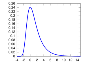
Probability density function [[File:350px $\mu =0,c=\pi /2$|frameless]]
Parameters	$c\in (0,\mathrm{\infty })$ — scale parameter $\mu \in (-\mathrm{\infty },\mathrm{\infty })$ — location parameter
Support	$\mathbb{ℝ}$
PDF	$\frac{1}{\pi c}\underset{0}{\overset{\mathrm{\infty }}{\int }}{e}^{-t}\cos ((x-\mu )\frac{t}{c}+\frac{2t}{\pi }\ln \frac{t}{c})dt$
Mean	Undefined
Variance	Undefined
MGF	Undefined
CF	$\exp (it\mu -\frac{2ict}{\pi }\log |t|-c|t|)$

In probability theory, the Landau distribution is a probability distribution named after Lev Landau who used it in 1944.

Because of the distribution's "fat" tail, the moments of the distribution, such as mean or variance, are undefined. The distribution is a particular case of stable distribution.

Definition

The probability density function, as written originally by Landau, is defined by the complex integral:

$$p(x)=\frac{1}{2\pi i}\underset{a-i\mathrm{\infty }}{\overset{a+i\mathrm{\infty }}{\int }}{e}^{s\ln s+xs}ds,$$

where a is an arbitrary positive real number, meaning that the integration path can be any parallel to the imaginary axis, intersecting the real positive semi-axis, and $\ln$ refers to the natural logarithm. In other words, it is the inverse Laplace transform of the function $s^s$.

The following real integral is equivalent to the above:

$$p(x)=\frac{1}{\pi }\underset{0}{\overset{\mathrm{\infty }}{\int }}{e}^{-t\ln t-xt}\sin (\pi t)dt.$$

The full family of Landau distributions is obtained by extending the original distribution to a location-scale family of stable distributions with parameters $\alpha =1$ and $\beta =1$, with characteristic function:

$$\phi (t;\mu ,c)=\exp (it\mu -\frac{2ict}{\pi }\ln |t|-c|t|)$$

where $c\in (0,\mathrm{\infty })$ and $\mu \in (-\mathrm{\infty },\mathrm{\infty })$, which yields a density function:

$$p(x;\mu ,c)=\frac{1}{\pi c}\underset{0}{\overset{\mathrm{\infty }}{\int }}{e}^{-t}\cos ((x-\mu )\frac{t}{c}+\frac{2t}{\pi }\ln \frac{t}{c})dt,$$

Taking $\mu =0$ and $c=\frac{\pi }{2}$ we get the original form of $p(x)$ above.

Properties

The approximation function for $\mu =0,c=1$

• Translation: If $X\sim \text{<mrow data-mjx-texclass="ORD">Landau</mrow>}(\mu ,c)$ then $X+m\sim \text{<mrow data-mjx-texclass="ORD">Landau</mrow>}(\mu +m,c)$.
• Scaling: If $X\sim \text{<mrow data-mjx-texclass="ORD">Landau</mrow>}(\mu ,c)$ then $aX\sim \text{<mrow data-mjx-texclass="ORD">Landau</mrow>}(a\mu -\frac{2}{\pi }ac\ln a,ac)$.
• Sum: If $X\sim \text{<mrow data-mjx-texclass="ORD">Landau</mrow>}({\mu }_1,c_1)$ and $Y\sim \text{<mrow data-mjx-texclass="ORD">Landau</mrow>}({\mu }_2,c_2)$ then $X+Y\sim \text{<mrow data-mjx-texclass="ORD">Landau</mrow>}({\mu }_1+{\mu }_2,c_1+c_2)$.

These properties can all be derived from the characteristic function. Together they imply that the Landau distributions are closed under affine transformations.

Approximations

In the "standard" case $\mu =0$ and $c=\pi /2$, the pdf can be approximated using Lindhard theory which says:

$$p(x+\ln x-1+\gamma )\approx \frac{\exp (-1/x)}{x(1+x)},$$

where $\gamma$ is Euler's constant.

A similar approximation of $p(x;\mu ,c)$ for $\mu =0$ and $c=1$ is:

$$p(x)\approx \frac{1}{\sqrt{2\pi }}\exp (-\frac{x+e^{-x}}{2}).$$

Applications

In nuclear and particle physics, the Landau distribution appears as a probability that a fast particle with a given initial energy will lose a given energy after passing the layer of matter with given thickness.

Related distributions

• The Landau distribution is a stable distribution with stability parameter $\alpha$ and skewness parameter $\beta$ both equal to 1.

References

- ↑ Landau, L. (1944). "On the energy loss of fast particles by ionization". J. Phys. (USSR) 8: 201. http://e-heritage.ru/Book/10093344.
- ↑ Gentle, James E. (2003). Random Number Generation and Monte Carlo Methods. Statistics and Computing (2nd ed.). New York, NY: Springer. p. 196. doi:10.1007/b97336. ISBN 978-0-387-00178-4.
- ↑ Zolotarev, V.M. (1986). One-dimensional stable distributions. Providence, R.I.: American Mathematical Society. ISBN 0-8218-4519-5. https://archive.org/details/onedimensionalst00zolo_0.
- ↑ "LandauDistribution—Wolfram Language Documentation". https://reference.wolfram.com/language/ref/LandauDistribution.html.
- ↑ Behrens, S. E.; Melissinos, A.C.. Univ. of Rochester Preprint UR-776 (1981).
- ↑ Bulyak E., Shul'ga N. (2022). "Landau distribution of ionization losses: history, importance, extensions". arXiv:2209.06387 [physics.plasm-ph].