Mark and recapture
Mark and recapture is a method commonly used in ecology to estimate an animal population's size where it is impractical to count every individual.[1] A portion of the population is captured, marked, and released. Later, another portion will be captured and the number of marked individuals within the sample is counted. Since the number of marked individuals within the second sample should be proportional to the number of marked individuals in the whole population, an estimate of the total population size can be obtained by dividing the number of marked individuals by the proportion of marked individuals in the second sample. Other names for this method, or closely related methods, include capture-recapture, capture-mark-recapture, mark-recapture, sight-resight, mark-release-recapture, multiple systems estimation, band recovery, the Petersen method,[2] and the Lincoln method.
Another major application for these methods is in epidemiology,[3] where they are used to estimate the completeness of ascertainment of disease registers. Typical applications include estimating the number of people needing particular services (i.e. services for children with learning disabilities, services for medically frail elderly living in the community), or with particular conditions (i.e. illegal drug addicts, people infected with HIV, etc.).[4]
Field work related to mark-recapture

Typically a researcher visits a study area and uses traps to capture a group of individuals alive. Each of these individuals is marked with a unique identifier (e.g., a numbered tag or band), and then is released unharmed back into the environment. A mark-recapture method was first used for ecological study in 1896 by C.G. Johannes Petersen to estimate plaice, Pleuronectes platessa, populations.[5]
Sufficient time is allowed to pass for the marked individuals to redistribute themselves among the unmarked population.[5]
Next, the researcher returns and captures another sample of individuals. Some individuals in this second sample will have been marked during the initial visit and are now known as recaptures.[6] Other organisms captured during the second visit, will not have been captured during the first visit to the study area. These unmarked animals are usually given a tag or band during the second visit and then are released.[5]
Population size can be estimated from as few as two visits to the study area. Commonly, more than two visits are made, particularly if estimates of survival or movement are desired. Regardless of the total number of visits, the researcher simply records the date of each capture of each individual. The "capture histories" generated are analyzed mathematically to estimate population size, survival, or movement.[5]
When capturing and marking organisms, ecologists need to consider the welfare of the organisms. If the chosen identifier harms the organism, then its behavior might become irregular.
-
 Collar-tagged rock hyrax
 -
 Ring-tagged Jackdaw
 -
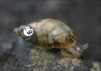 Marked Chittenango ovate amber snail
 -
 Tagged Common Ringlet


Notation
Let
- N = Number of animals in the population
- n = Number of animals marked on the first visit
- K = Number of animals captured on the second visit
- k = Number of recaptured animals that were marked
A biologist wants to estimate the size of a population of turtles in a lake. She captures 10 turtles on her first visit to the lake, and marks their backs with paint. A week later she returns to the lake and captures 15 turtles. Five of these 15 turtles have paint on their backs, indicating that they are recaptured animals. This example is (n, K, k) = (10, 15, 5). The problem is to estimate N.
Lincoln–Petersen estimator
The Lincoln–Petersen method[7] (also known as the Petersen–Lincoln index[5] or Lincoln index) can be used to estimate population size if only two visits are made to the study area. This method assumes that the study population is "closed". In other words, the two visits to the study area are close enough in time so that no individuals die, are born, or move into or out of the study area between visits. The model also assumes that no marks fall off animals between visits to the field site by the researcher, and that the researcher correctly records all marks.
Given those conditions, estimated population size is:
Derivation
It is assumed[8] that all individuals have the same probability of being captured in the second sample, regardless of whether they were previously captured in the first sample (with only two samples, this assumption cannot be tested directly).
This implies that, in the second sample, the proportion of marked individuals that are caught () should equal the proportion of the total population that is marked (). For example, if half of the marked individuals were recaptured, it would be assumed that half of the total population was included in the second sample.
In symbols,
A rearrangement of this gives
the formula used for the Lincoln–Petersen method.[8]
Sample calculation
In the example (n, K, k) = (10, 15, 5) the Lincoln–Petersen method estimates that there are 30 turtles in the lake.
Chapman estimator
The Lincoln–Petersen estimator is asymptotically unbiased as sample size approaches infinity, but is biased at small sample sizes.[9] An alternative less biased estimator of population size is given by the Chapman estimator:[9]
Sample calculation
The example (n, K, k) = (10, 15, 5) gives
Note that the answer provided by this equation must be truncated not rounded. Thus, the Chapman method estimates 28 turtles in the lake.
Surprisingly, Chapman's estimate was one conjecture from a range of possible estimators: "In practice, the whole number immediately less than (K+1)(n+1)/(k+1) or even Kn/(k+1) will be the estimate. The above form is more convenient for mathematical purposes."[9](see footnote, page 144). Chapman also found the estimator could have considerable negative bias for small Kn/N [9](page 146), but was unconcerned because the estimated standard deviations were large for these cases.
Confidence interval
An approximate confidence interval for the population size N can be obtained as:
where corresponds to the quantile of a standard normal random variable, and
The example (n, K, k) = (10, 15, 5) gives the estimate N ≈ 30 with a 95% confidence interval of 22 to 65.
It has been shown that this confidence interval has actual coverage probabilities that are close to the nominal level even for small populations and extreme capture probabilities (near to 0 or 1), in which cases other confidence intervals fail to achieve the nominal coverage levels.[10]
Bayesian estimate
The mean value ± standard deviation is
where
- for
- for
A derivation is found here: Talk:Mark and recapture#Statistical treatment.
The example (n, K, k) = (10, 15, 5) gives the estimate N ≈ 42 ± 21.5
Capture probability

The capture probability refers to the probability of a detecting an individual animal or person of interest,[11] and has been used in both ecology and epidemiology for detecting animal or human diseases,[12] respectively.
The capture probability is often defined as a two-variable model, in which f is defined as the fraction of a finite resource devoted to detecting the animal or person of interest from a high risk sector of an animal or human population, and q is the frequency of time that the problem (e.g., an animal disease) occurs in the high-risk versus the low-risk sector.[13] For example, an application of the model in the 1920s was to detect typhoid carriers in London, who were either arriving from zones with high rates of tuberculosis (probability q that a passenger with the disease came from such an area, where q>0.5), or low rates (probability 1−q).[14] It was posited that only 5 out of every 100 of the travelers could be detected, and 10 out of every 100 were from the high risk area. Then the capture probability P was defined as:
where the first term refers to the probability of detection (capture probability) in a high risk zone, and the latter term refers to the probability of detection in a low risk zone. Importantly, the formula can be re-written as a linear equation in terms of f:
Because this is a linear function, it follows that for certain versions of q for which the slope of this line (the first term multiplied by f) is positive, all of the detection resource should be devoted to the high-risk population (f should be set to 1 to maximize the capture probability), whereas for other value of q, for which the slope of the line is negative, all of the detection should be devoted to the low-risk population (f should be set to 0. We can solve the above equation for the values of q for which the slope will be positive to determine the values for which f should be set to 1 to maximize the capture probability:
which simplifies to:
This is an example of linear optimization.[13] In more complex cases, where more than one resource f is devoted to more than two areas, multivariate optimization is often used, through the simplex algorithm or its derivatives.
More than two visits
The literature on the analysis of capture-recapture studies has blossomed since the early 1990s[citation needed]. There are very elaborate statistical models available for the analysis of these experiments.[15] A simple model which easily accommodates the three source, or the three visit study, is to fit a Poisson regression model. Sophisticated mark-recapture models can be fit with several packages for the Open Source R programming language. These include "Spatially Explicit Capture-Recapture (secr)",[16] "Loglinear Models for Capture-Recapture Experiments (Rcapture)",[17] and "Mark-Recapture Distance Sampling (mrds)".[18] Such models can also be fit with specialized programs such as MARK[19] or E-SURGE.[20]
Other related methods which are often used include the Jolly–Seber model (used in open populations and for multiple census estimates) and Schnabel estimators[21] (an expansion to the Lincoln–Petersen method for closed populations). These are described in detail by Sutherland.[22]
Integrated approaches
Modelling mark-recapture data is trending towards a more integrative approach,[23] which combines mark-recapture data with population dynamics models and other types of data. The integrated approach is more computationally demanding, but extracts more information from the data improving parameter and uncertainty estimates.[24]
See also
- German tank problem, for estimation of population size when the elements are numbered.
- Tag and release
- Abundance estimation
- GPS wildlife tracking
- Shadow Effect (Genetics)
References
- ↑ "Mark-Recapture". http://www2.nau.edu/lrm22/lessons/mark_recapture/mark_recapture.html.
- ↑ Krebs, Charles J. (2009). Ecology (6th ed.). Pearson Benjamin Cummings. p. 119. ISBN 978-0-321-50743-3.
- ↑ Chao, A.; Tsay, P. K.; Lin, S. H.; Shau, W. Y.; Chao, D. Y. (2001). "The applications of capture-recapture models to epidemiological data". Statistics in Medicine 20 (20): 3123–3157. doi:10.1002/sim.996. PMID 11590637.
- ↑ Allen (2019). "Estimating the Number of People Who Inject Drugs in A Rural County in Appalachia". American Journal of Public Health 109 (3): 445–450. doi:10.2105/AJPH.2018.304873. PMID 30676803.
- ↑ 5.0 5.1 5.2 5.3 5.4 Southwood, T. R. E.; Henderson, P. (2000). Ecological Methods (3rd ed.). Oxford: Blackwell Science.
- ↑ "Recapture Definition & Meaning - Merriam-Webster". 21 August 2023. https://www.merriam-webster.com/dictionary/recapture.
- ↑ Seber, G. A. F. (1982). The Estimation of Animal Abundance and Related Parameters. Caldwel, New Jersey: Blackburn Press. ISBN 1-930665-55-5.
- ↑ 8.0 8.1 Charles J. Krebs (1999). Ecological Methodology (2nd ed.). Benjamin/Cummings. ISBN 9780321021731. https://books.google.com/books?id=1GwVAQAAIAAJ.
- ↑ 9.0 9.1 9.2 9.3 Chapman, D.G. (1951). Some properties of the hypergeometric distribution with applications to zoological sample censuses.
- ↑ Sadinle, Mauricio (2009-10-01). "Transformed Logit Confidence Intervals for Small Populations in Single Capture–Recapture Estimation". Communications in Statistics - Simulation and Computation 38 (9): 1909–1924. doi:10.1080/03610910903168595. ISSN 0361-0918.
- ↑ Drenner, Ray (1978). "Capture probability: the role of zooplankter escape in the selective feeding of planktivorous fish". Journal of the Fisheries Board of Canada 35 (10): 1370–1373. doi:10.1139/f78-215.
- ↑ MacKenzie, Darryl (2002). "How should detection probability be incorporated into estimates of relative abundance?". Ecology 83 (9): 2387–2393. doi:10.1890/0012-9658(2002)083[2387:hsdpbi2.0.co;2].
- ↑ 13.0 13.1 Bolker, Benjamin (2008). Ecological Models and Data in R. Princeton University Press. ISBN 9781400840908.
- ↑ Unknown (1921). "The Health of London". Hosp Health Rev 1 (3): 71–2. PMID 29418259.
- ↑ McCrea, R.S. and Morgan, B.J.T. (2014) "Analysis of capture-recapture data.". http://www.capturerecapture.co.uk. "Chapman and Hall/CRC Press". http://www.crcpress.com/product/isbn/9781439836590.
- ↑ Efford, Murray (2016-09-02). "Spatially Explicit Capture-Recapture (secr)". Comprehensive R Archive Network (CRAN). https://cran.r-project.org/web/packages/secr/index.html.
- ↑ Rivest, Louis-Paul; Baillargeon, Sophie (2014-09-01). "Loglinear Models for Capture-Recapture Experiments (Rcapture)". Comprehensive R Archive Network (CRAN). https://cran.r-project.org/web/packages/Rcapture/index.html.
- ↑ Laake, Jeff; Borchers, David; Thomas, Len; Miller, David; Bishop, Jon (2015-08-17). "Mark-Recapture Distance Sampling (mrds)". Comprehensive R Archive Network (CRAN). https://cran.r-project.org/web/packages/mrds/index.html.
- ↑ "Program MARK". http://www.warnercnr.colostate.edu/~gwhite/mark/mark.htm.
- ↑ "Logiciels". http://www.cefe.cnrs.fr/biom/Logiciels.htm.
- ↑ Schnabel, Z. E. (1938). "The Estimation of the Total Fish Population of a Lake". American Mathematical Monthly 45 (6): 348–352. doi:10.2307/2304025.
- ↑ William J. Sutherland, ed (1996). Ecological Census Techniques: A Handbook. Cambridge University Press. ISBN 0-521-47815-4.
- ↑ Maunder M.N. (2003) Paradigm shifts in fisheries stock assessment: from integrated analysis to Bayesian analysis and back again. Natural Resource Modeling 16:465–475
- ↑ Maunder, M.N. (2001) Integrated Tagging and Catch-at-Age Analysis (ITCAAN). In Spatial Processes and Management of Fish Populations, edited by G.H. Kruse, N. Bez, A. Booth, M.W. Dorn, S. Hills, R.N. Lipcius, D. Pelletier, C. Roy, S.J. Smith, and D. Witherell, Alaska Sea Grant College Program Report No. AK-SG-01-02, University of Alaska Fairbanks, pp. 123–146.
- Besbeas, P; Freeman, S. N.; Morgan, B. J. T.; Catchpole, E. A. (2002). "Integrating mark-recapture-recovery and census data to estimate animal abundance and demographic parameters.". Biometrics 58 (3): 540–547. doi:10.1111/j.0006-341X.2002.00540.x. PMID 12229988.
- "Mortality rate calculations on ringed birds with special reference to the Dunlin Calidris alpina". Arkiv för Zoologi (Zoology Files), Kungliga Svenska Vetenskapsakademien (The Royal Swedish Academy of Sciences) Serie 2 Band 13 (21). 1961.
- Maunder, M. N. (2004). "Population viability analysis, based on combining integrated, Bayesian, and hierarchical analyses". Acta Oecologica 26 (2): 85–94. doi:10.1016/j.actao.2003.11.008. Bibcode: 2004AcO....26...85M.
- Phillips, C. A.; M. J. Dreslik; J. R. Johnson; J. E. Petzing (2001). "Application of population estimation to pond breeding salamanders". Transactions of the Illinois Academy of Science 94 (2): 111–118.
- Royle, J. A.; R. M. Dorazio (2008). Hierarchical Modeling and Inference in Ecology. Elsevier. ISBN 978-1-930665-55-2.
- Seber, G.A.F. (2002). The Estimation of Animal Abundance and Related Parameters. Caldwel, New Jersey: Blackburn Press. ISBN 1-930665-55-5.
- Schaub, M; Gimenez, O.; Sierro, A.; Arlettaz, R (2007). "Use of Integrated Modeling to Enhance Estimates of Population Dynamics Obtained from Limited Data". Conservation Biology 21 (4): 945–955. doi:10.1111/j.1523-1739.2007.00743.x. PMID 17650245. Bibcode: 2007ConBi..21..945S. https://hal.archives-ouvertes.fr/hal-03515125/file/06-425schaub-MS%20-%20OG.pdf.
- Williams, B. K.; J. D. Nichols; M. J. Conroy (2002). Analysis and Management of Animal Populations. San Diego, California: Academic Press. ISBN 0-12-754406-2.
- Chao, A; Tsay, P. K.; Lin, S. H.; Shau, W. Y.; Chao, D. Y. (2001). "The applications of capture-recapture models to epidemiological data". Statistics in Medicine 20 (20): 3123–3157. doi:10.1002/sim.996. PMID 11590637.
Further reading
- Bonett, D.G.; Woodward, J.A.; Bentler, P.M. (1986). "A Linear Model for Estimating the Size of a Closed Population". British Journal of Mathematical and Statistical Psychology 39: 28–40. doi:10.1111/j.2044-8317.1986.tb00843.x. PMID 3768264.
- Evans, M.A.; Bonett, D.G.; McDonald, L. (1994). "A General Theory for Analyzing Capture-recapture Data in Closed Populations". Biometrics 50 (2): 396–405. doi:10.2307/2533383.
- Lincoln, F. C. (1930). "Calculating Waterfowl Abundance on the Basis of Banding Returns". United States Department of Agriculture Circular 118: 1–4.
- Petersen, C. G. J. (1896). "The Yearly Immigration of Young Plaice Into the Limfjord From the German Sea", Report of the Danish Biological Station (1895), 6, 5–84.
- Schofield, J. R. (2007). "Beyond Defect Removal: Latent Defect Estimation With Capture-Recapture Method", Crosstalk, August 2007; 27–29.
External links
 |  |

