Maximum subarray problem

In computer science, the maximum sum subarray problem, also known as the maximum segment sum problem, is the task of finding a contiguous subarray with the largest sum, within a given one-dimensional array A[1...n] of numbers. It can be solved in time and space.
Formally, the task is to find indices and with , such that the sum
is as large as possible. (Some formulations of the problem also allow the empty subarray to be considered; by convention, the sum of all values of the empty subarray is zero.) Each number in the input array A could be positive, negative, or zero.[1]
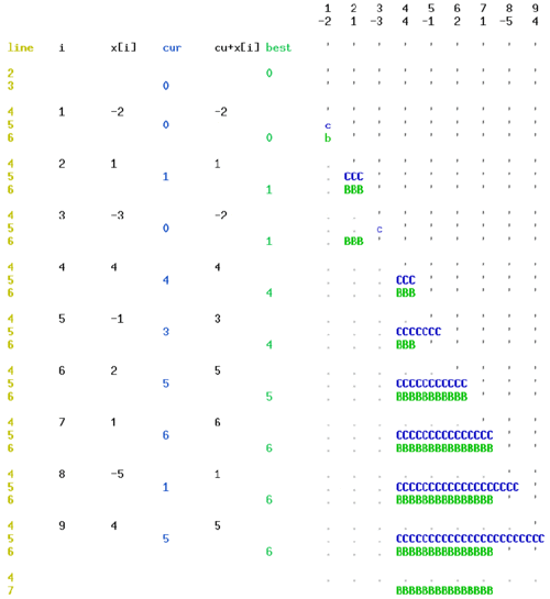
For example, for the array of values [−2, 1, −3, 4, −1, 2, 1, −5, 4], the contiguous subarray with the largest sum is [4, −1, 2, 1], with sum 6.
Some properties of this problem are:
- If the array contains all non-negative numbers, then the problem is trivial; a maximum subarray is the entire array.
- If the array contains all non-positive numbers, then a solution is any subarray of size 1 containing the maximal value of the array (or the empty subarray, if it is permitted).
- Several different sub-arrays may have the same maximum sum.
Although this problem can be solved using several different algorithmic techniques, including brute force,[2] divide and conquer,[3] dynamic programming,[4] and reduction to shortest paths, a simple single-pass algorithm known as Kadane's algorithm solves it efficiently.
History
The maximum subarray problem was proposed by Ulf Grenander in 1977 as a simplified model for maximum likelihood estimation of patterns in digitized images.[5]
Grenander was looking to find a rectangular subarray with maximum sum, in a two-dimensional array of real numbers. A brute-force algorithm for the two-dimensional problem runs in O(n6) time; because this was prohibitively slow, Grenander proposed the one-dimensional problem to gain insight into its structure. Grenander derived an algorithm that solves the one-dimensional problem in O(n2) time using prefix sums[note 1], improving the brute force running time of O(n3). When Michael Shamos heard about the problem, he overnight devised an O(n log n) divide-and-conquer algorithm for it. Soon after, Shamos described the one-dimensional problem and its history at a Carnegie Mellon University seminar attended by Jay Kadane, who designed within a minute an O(n)-time algorithm,[5][6][7] which is as fast as possible.[note 2] In 1982, David Gries obtained the same O(n)-time algorithm by applying Dijkstra's "standard strategy";[8] in 1989, Richard Bird derived it by purely algebraic manipulation of the brute-force algorithm using the Bird–Meertens formalism.[9]
Grenander's two-dimensional generalization can be solved in O(n3) time either by using Kadane's algorithm as a subroutine, or through a divide-and-conquer approach. Slightly faster algorithms based on distance matrix multiplication have been proposed by (Tamaki Tokuyama) and by (Takaoka 2002). There is some evidence that no significantly faster algorithm exists; an algorithm that solves the two-dimensional maximum subarray problem in O(n3−ε) time, for any ε>0, would imply a similarly fast algorithm for the all-pairs shortest paths problem.[10]
Applications
Maximum subarray problems arise in many fields, such as genomic sequence analysis and computer vision.
Genomic sequence analysis employs maximum subarray algorithms to identify important biological segments of protein sequences that have unusual properties, by assigning scores to points within the sequence that are positive when a motif to be recognized is present, and negative when it is not, and then seeking the maximum subarray among these scores. These problems include conserved segments, GC-rich regions, tandem repeats, low-complexity filter, DNA binding domains, and regions of high charge.[11]
In computer vision, bitmap images generally consist only of positive values, for which the maximum subarray problem is trivial: the result is always the whole array. However, after subtracting a threshold value (such as the average pixel value) from each pixel, so that above-average pixels will be positive and below-average pixels will be negative, the maximum subarray problem can be applied to the modified image to detect bright areas within it.[12]
Kadane's algorithm
No empty subarrays admitted
Kadane's algorithm scans the given array from left to right.
In the th step, it computes the subarray with the largest sum ending at ; this sum is maintained in variable current_sum.[note 3]
Moreover, it computes the subarray with the largest sum anywhere in , maintained in variable best_sum,[note 4]
and easily obtained as the maximum of all values of current_sum seen so far, cf. line 7 of the algorithm.
As a loop invariant, in the th step, the old value of current_sum holds the maximum over all of the sum .
Therefore, current_sum[note 5]
is the maximum over all of the sum . To extend the latter maximum to also cover the case , it is sufficient to also consider the singleton subarray . This is done in line 6 by assigning current_sum as the new value of current_sum, which after that holds the maximum over all of the sum .
Thus, the problem can be solved with the following code,[13] expressed in Python.
def max_subarray(numbers):
    """Find the largest sum of any contiguous subarray."""
    best_sum = float('-inf')
    current_sum = 0
    for x in numbers:
        current_sum = max(x, current_sum + x)
        best_sum = max(best_sum, current_sum)
    return best_sum
If the input contains no positive element, the returned value is that of the largest element (i.e., the value closest to 0), or negative infinity if the input was empty. For correctness, an exception should be raised when the input array is empty, since an empty array has no maximum nonempty subarray. If the array is nonempty, its first element could be used in place of negative infinity, if needed to avoid mixing numeric and non-numeric values.
The algorithm can be adapted to the case which allows empty subarrays or to keep track of the starting and ending indices of the maximum subarray.
This algorithm calculates the maximum subarray ending at each position from the maximum subarray ending at the previous position, so it can be viewed as a case of dynamic programming.
Empty subarrays admitted
| Example run |
|---|
 |
Kadane's algorithm, as originally published, is for solving the problem variant which allows empty subarrays.[4][7]
In such a variant, the answer is 0 when the input contains no positive elements (including when the input is empty).
The variant is obtained with two changes in code: in line 3, best_sum should be initialized to 0 to account for the empty subarray
best_sum = 0;
and line 6 in the for loop current_sum should be updated to max(0, current_sum + x).[note 6]
current_sum = max(0, current_sum + x)
As a loop invariant, in the th step, the old value of current_sum holds the maximum over all of the sum .[note 7]
Therefore, current_sum
is the maximum over all of the sum . To extend the latter maximum to also cover the case , it is sufficient to also consider the empty subarray . This is done in line 6 by assigning current_sum as the new value of current_sum, which after that holds the maximum over all of the sum . Machine-verified C / Frama-C code of both variants can be found here.
Computing the best subarray's position
The algorithm can be modified to keep track of the starting and ending indices of the maximum subarray as well.
Because of the way this algorithm uses optimal substructures (the maximum subarray ending at each position is calculated in a simple way from a related but smaller and overlapping subproblem: the maximum subarray ending at the previous position) this algorithm can be viewed as a simple/trivial example of dynamic programming.
Complexity
The runtime complexity of Kadane's algorithm is and its space complexity is .[4][7]
Generalizations
Similar problems may be posed for higher-dimensional arrays, but their solutions are more complicated; see, e.g., (Takaoka 2002). (Brodal Jørgensen) showed how to find the k largest subarray sums in a one-dimensional array, in the optimal time bound .
The Maximum sum k-disjoint subarrays can also be computed in the optimal time bound .[14]
See also
Notes
- ↑ By using a precomputed table of cumulative sums to compute the subarray sum in constant time
- ↑ since every algorithm must at least scan the array once which already takes O(n) time
- ↑ named
MaxEndingHerein (Bentley 1989), andcin (Gries 1982) - ↑ named
MaxSoFarin (Bentley 1989), andsin (Gries 1982) - ↑
In the Python code below, is expressed as
x, with the index left implicit. - ↑ While (Bentley 1989) does not mention this difference, using
xinstead of0in the above version without empty subarrays achieves maintaining its loop invariantcurrent_sumat the beginning of the th step. - ↑ This sum is when , corresponding to the empty subarray .
Notes
- ↑ Bentley 1989, p. 69.
- ↑ Bentley 1989, p. 70.
- ↑ Bentley 1989, p. 73.
- ↑ 4.0 4.1 4.2 Bentley 1989, p. 74.
- ↑ 5.0 5.1 Bentley 1984, p. 868-869.
- ↑ Bentley 1989, p. 76-77.
- ↑ 7.0 7.1 7.2 Gries 1982, p. 211.
- ↑ Gries 1982, p. 209-211.
- ↑ Bird 1989, Sect.8, p.126.
- ↑ Backurs, Dikkala & Tzamos 2016.
- ↑ (Ruzzo Tompa); (Alves Cáceres)
- ↑ (Bae Takaoka); (Weddell Read)
- ↑ Bentley 1989, p. 78,171. Bentley, like Gries, first introduces the variant admitting empty subarrays, see below, and describes only the changes.
- ↑ Bengtsson & Chen 2007.
References
- Alves, Carlos E. R.; Cáceres, Edson; Song, Siang W. (2004), "BSP/CGM Algorithms for Maximum Subsequence and Maximum Subarray", in Kranzlmüller, Dieter; Kacsuk, Péter; Dongarra, Jack J., Recent Advances in Parallel Virtual Machine and Message Passing Interface, 11th European PVM/MPI Users' Group Meeting, Budapest, Hungary, September 19-22, 2004, Proceedings, Lecture Notes in Computer Science, 3241, Springer, pp. 139–146, doi:10.1007/978-3-540-30218-6_24, ISBN 978-3-540-23163-9
- Backurs, Arturs; Dikkala, Nishanth; Tzamos, Christos (2016), "Tight Hardness Results for Maximum Weight Rectangles", 43rd International Colloquium on Automata, Languages, and Programming (ICALP 2016), Leibniz International Proceedings in Informatics (LIPIcs), 55, Schloss Dagstuhl – Leibniz-Zentrum für Informatik, pp. 81:1–81:13, doi:10.4230/LIPIcs.ICALP.2016.81, ISBN 978-3-95977-013-2
- Bae, Sung Eun (2007), Sequential and Parallel Algorithms for the Generalized Maximum Subarray Problem, https://pdfs.semanticscholar.org/bea4/1795adaf240b9db4195b9dc511bd8d46bff1.pdf.
- Bae, Sung Eun; Takaoka, Tadao (2006), "Improved Algorithms for the \emph{K}-Maximum Subarray Problem", The Computer Journal 49 (3): 358–374, doi:10.1093/COMJNL/BXL007
- Bengtsson, Fredrik; Chen, Jingsen (2007), Computing maximum-scoring segments optimally, http://ltu.diva-portal.org/smash/get/diva2:995901/FULLTEXT01.pdf
- Bentley, Jon (1984), "Programming Pearls: Algorithm Design Techniques", Communications of the ACM 27 (9): 865–873, doi:10.1145/358234.381162
- Bentley, Jon (May 1989), Programming Pearls (2nd? ed.), Reading, MA: Addison Wesley, ISBN 0-201-10331-1, https://archive.org/details/programmingpearl00bent
- Bird, Richard S. (1989), "Algebraic Identities for Program Calculation", The Computer Journal 32 (2): 122–126, doi:10.1093/comjnl/32.2.122
- Brodal, Gerth Stølting; Jørgensen, Allan Grønlund (2007), "A linear time algorithm for the k maximal sums problem", Mathematical Foundations of Computer Science 2007, Lecture Notes in Computer Science, 4708, Springer-Verlag, pp. 442–453, doi:10.1007/978-3-540-74456-6_40, ISBN 978-3-540-74455-9.
- Gries, David (1982), "A Note on the Standard Strategy for Developing Loop Invariants and Loops", Science of Computer Programming 2 (3): 207–241, doi:10.1016/0167-6423(83)90015-1, https://core.ac.uk/download/pdf/82596333.pdf
- Ruzzo, Walter L.; Tompa, Martin (1999), "A Linear Time Algorithm for Finding All Maximal Scoring Subsequences", in Lengauer, Thomas; Schneider, Reinhard; Bork, Peer et al., Proceedings of the Seventh International Conference on Intelligent Systems for Molecular Biology, August 6–10, 1999, Heidelberg, Germany, AAAI, pp. 234–241, https://www.aaai.org/Library/ISMB/1999/ismb99-027.php
- Takaoka, Tadao (2002), "Efficient algorithms for the maximum subarray problem by distance matrix multiplication", Electronic Notes in Theoretical Computer Science 61: 191–200, doi:10.1016/S1571-0661(04)00313-5.
- Tamaki, Hisao; Tokuyama, Takeshi (1998), "Algorithms for the Maximum Subarray Problem Based on Matrix Multiplication", Proceedings of the 9th Symposium on Discrete Algorithms (SODA): 446–452, ISBN 978-0-89871-410-4, http://dl.acm.org/citation.cfm?id=314613.314823, retrieved November 17, 2018
- Weddell, Stephen John; Read, Tristan; Thaher, Mohammed; Takaoka, Tadao (2013), "Maximum subarray algorithms for use in astronomical imaging", Journal of Electronic Imaging 22 (4), doi:10.1117/1.JEI.22.4.043011, Bibcode: 2013JEI....22d3011W
External links
- TAN, Lirong. "Maximum Contiguous Subarray Sum Problems". http://www.picb.ac.cn/~xiaohang/vimwiki/study/tanlirong/Algorithm/project/Report.pdf.
- Mu, Shin-Cheng (2010). "The Maximum Segment Sum Problem: Its Origin, and a Derivation". https://www.iis.sinica.edu.tw/~scm/2010/maximum-segment-sum-origin-and-derivation.
- "Notes on Maximum Subarray Problem". 2012. http://cs.slu.edu/~goldwamh/courses/slu/csci314/2012_Fall/lectures/maxsubarray/.
- www.algorithmist.com
- alexeigor.wikidot.com
- greatest subsequential sum problem on Rosetta Code
- geeksforgeeks page on Kadane's Algorithm
 |
