Multi-fractional order estimator

The multi-fractional order estimator (MFOE) is a straightforward, practical, and flexible alternative to the Kalman filter (KF) for tracking targets. The MFOE is focused strictly on simple and pragmatic fundamentals along with the integrity of mathematical modeling. Like the KF, the MFOE is based on the least squares method (LSM) invented by Gauss and the orthogonality principle at the center of Kalman's derivation. Optimized, the MFOE yields better accuracy than the KF and subsequent algorithms such as the extended KF and the interacting multiple model (IMM). The MFOE is an expanded form of the LSM, which effectively includes the KF and ordinary least squares (OLS) as subsets (special cases). OLS is revolutionized in for application in econometrics. The MFOE also intersects with signal processing, estimation theory, economics, finance, statistics, and the method of moments. The MFOE offers two major advances: (1) minimizing the mean squared error (MSE) with fractions of estimated coefficients (useful in target tracking) and (2) describing the effect of deterministic OLS processing of statistical inputs (of value in econometrics)

Description

Consider equally time spaced noisy measurement samples of a target trajectory described by

[math]\displaystyle{ y_n = \sum_{j=1} ^J c_j n^{j-1} + \eta_n= x_n + \eta_n }[/math]

where n represents both the time samples and the index; the polynomial describing the trajectory is of degree J-1; and [math]\displaystyle{ \eta_n }[/math] is zero mean, stationary, white noise (not necessarily Gaussian) with variance [math]\displaystyle{ \sigma_n ^2 }[/math].

Estimating x(t) at time [math]\displaystyle{ \tau }[/math] with the MFOE is described by

[math]\displaystyle{ \hat x (\tau) = \sum_{n=1}^{N} y_n w_n (\tau) }[/math]

where the hat (^) denotes an estimate, N is the number of samples in the data window, [math]\displaystyle{ \tau }[/math] is the time of the desired estimate, and the data weights are

[math]\displaystyle{ w_n (\tau) = \sum _m U_{mn} T_m (\tau) f_m }[/math]

The [math]\displaystyle{ U_{mn} }[/math] are orthogonal polynomial coefficient estimators. [math]\displaystyle{ T_{m}(\tau) }[/math] (a function detailed in) projects the estimate of the polynomial coefficient [math]\displaystyle{ c_m }[/math] to the desired estimation time [math]\displaystyle{ \tau }[/math]. The MFOE parameter 0≤[math]\displaystyle{ f_m }[/math]≤1 can apply a fraction of the projected coefficient estimate.

The combined terms [math]\displaystyle{ U_{mn}T_m }[/math] effectively constitute a novel set of expansion functions with coefficients [math]\displaystyle{ f_m }[/math]. The MFOE can be optimized at time [math]\displaystyle{ \tau }[/math] as a function of the [math]\displaystyle{ f_m }[/math]s for given measurement noise, target dynamics, and non-recursive sliding data window size, N. However, for all [math]\displaystyle{ f_m=1 }[/math], the MFOE reduces and is equivalent to the KF in the absence of process noise, and to the standard polynomial LSM.

As in the case of coefficients in conventional series expansions, the [math]\displaystyle{ f_m }[/math]s typically decrease monotonically as higher order terms are included to match complex target trajectories. For example, in the [math]\displaystyle{ f_m }[/math]s monotonically decreased in the MFOE from [math]\displaystyle{ f_1=1 }[/math] to [math]\displaystyle{ f_5 \gtrsim 0 }[/math] , where [math]\displaystyle{ f_m = 0 }[/math] for m ≧ 6. The MFOE in consisted of five point, 5th order processing of composite real (but altered for declassification) cruise missile data. A window of only 5 data points provided excellent maneuver following; whereas, 5th order processing included fractions of higher order terms to better approximate the complex maneuvering target trajectory. The MFOE overcomes the long-ago rejection of terms higher than 3rd order because, taken at full value (i.e., [math]\displaystyle{ f_{m}s=1 }[/math]), estimator variances increase exponentially with linear order increases. (This is elucidated below in the section "Application of the FOE".)

Fractional order estimator

As described in, the MFOE can be written more efficiently as [math]\displaystyle{ \hat x = \lt \psi,\omega_m\gt }[/math] where the estimator weights [math]\displaystyle{ w_n(\tau) }[/math] of order m are components of the estimating vector [math]\displaystyle{ \omega_m (\tau) }[/math]. By definition [math]\displaystyle{ \hat x \doteq \hat x(\tau) }[/math] and [math]\displaystyle{ \omega_m\doteq \omega_m(\tau) }[/math]. The angle brackets and comma [math]\displaystyle{ \lt ,\gt }[/math] denote the inner product, and the data vector [math]\displaystyle{ \psi }[/math] comprises noisy measurement samples [math]\displaystyle{ y_n }[/math].

Perhaps the most useful MFOE tracking estimator is the simple fractional order estimator (FOE) where [math]\displaystyle{ f_1=f_2=1 }[/math] and [math]\displaystyle{ f_m=0 }[/math] for all m > 3, leaving only [math]\displaystyle{ 0\le f_3 \le 1 }[/math]. This is effectively an FOE of fractional order [math]\displaystyle{ 2+f_3 }[/math], which linear interpolates between the 2nd and 3rd order estimators described in) as

[math]\displaystyle{ w_{2+f_{3}}=(1-f_3) \omega_2 +f_3 \omega_3 = \omega_2 + f_3 (\omega_3-\omega_2)=\omega_2+f_3\nu_3 }[/math]

where the scalar fraction [math]\displaystyle{ f_3 }[/math] is the linear interpolation factor, the vector [math]\displaystyle{ \nu_3=\omega_3-\omega_2= \upsilon_3T_3 }[/math], and [math]\displaystyle{ \upsilon_3 }[/math] (which comprises the components [math]\displaystyle{ U_{3n} }[/math]) is the vector estimator of the 3rd polynomial coefficient [math]\displaystyle{ c_3\equiv\tfrac{a\Delta^2}{2} }[/math] (a is acceleration and Δ is the sample period). The vector [math]\displaystyle{ \nu_3 }[/math] is the acceleration estimator from [math]\displaystyle{ \omega_3 }[/math].

The mean-square error (MSE) from the FOE applied to an accelerating target is

[math]\displaystyle{ MSE=\sigma_\eta ^2(|\omega_2|^2+f_3^2|\nu_3|^2)+[c_3T_3(1-f_3)]^2 }[/math], where for any vector [math]\displaystyle{ \theta }[/math], [math]\displaystyle{ | \theta |^2 \doteq\lt \theta,\theta\gt }[/math].

The first term on the right of the equal sign is the FOE target location estimator variance [math]\displaystyle{ \sigma_\eta ^2(|\omega_2|^2+f_3^2|\nu_3|^2) }[/math] composed of the 2nd order location estimator variance and part of the variance from the 3rd order acceleration estimator as determined by the interpolation factor squared [math]\displaystyle{ f_3^2 }[/math]. The second term is the bias squared [math]\displaystyle{ [c_3T_3(1-f_3)]^2 }[/math] from the 2nd order target location estimator as a function of acceleration in [math]\displaystyle{ c_3 }[/math].

Setting the derivative of the MSE with respect to [math]\displaystyle{ f_3 }[/math] equal to zero and solving yields the optimal [math]\displaystyle{ f_3 }[/math]:

[math]\displaystyle{ f_{3,opt} \doteq f_{3,opt}(\tau)= \frac {(c_3 T_3)^2} {(c_3 T_3)^2 + \sigma_\eta ^2 |\nu_3|^2} = \frac {c_3^2} {c_3^2 + \sigma_\eta^2|\upsilon_3|^2}= \frac {\rho_3^2} {\rho_3^2+|\upsilon_3|^2} }[/math]

where [math]\displaystyle{ \rho_3\equiv \frac {c_3}{\sigma_\eta}=\frac {a\Delta^2} {2\sigma_\eta} }[/math] , as defined in.

The optimal FOE is then very simply

[math]\displaystyle{ w_{2+f_{3,opt}}=\omega_2+f_{3,opt}\nu_3=\omega_2+\upsilon_3 T_3f_{3,opt}= \omega_2+\upsilon_3T_3\frac {\rho_3^2} {\rho_3^2+|\upsilon_3|^2} }[/math]

Substituting the optimal FOE into the MSE yields the minimum MSE:

[math]\displaystyle{ MSE_{min}=\sigma_\eta ^2(|\omega_2|^2+f_{3,opt}|\nu_3|^2) }[/math]

Although not obvious, the [math]\displaystyle{ MSE_{min} }[/math] includes the bias squared. The variance in the FOE MSE is the quadratic interpolation between the 2nd and the 3rd order location estimator variances as a function of [math]\displaystyle{ f_{3,opt}^2 }[/math]. Whereas, the [math]\displaystyle{ MSE_{min} }[/math] is the linear interpolation between the same 2nd and the 3rd order location estimator variances as a function of [math]\displaystyle{ f_{3,opt} }[/math]. The bias squared accounts for the difference.

Application of the FOE

Since a target's future location is generally of more interest than where it is or has been, consider one-step prediction. Normalized with respect to measurement noise variance, the MSE for equally spaced samples reduces for the predicted position to

[math]\displaystyle{ MSE = \frac {1} {N}+\frac {3(N+1)} {N(N-1)}+ f_3^2\frac {5(N+1)(N+2)}{N ((N-1)(N-2)}+\rho_3^2 \left [\frac {(N+1)(N+2)}{6}\right ] ^2 (1-f_3)^2 }[/math]

where N is the number of samples in the non-recursive sliding data window. Note that the first term on the right of the equal sign is the variance from estimating the first coefficient (position); the second term is the variance from estimating the 2nd coefficient (velocity); and the 3rd term with [math]\displaystyle{ f_3 = 1 }[/math] is the variance from estimating the 3rd coefficient (which includes acceleration). This pattern continues for higher order terms. Furthermore, the sum of the variances from estimating the first two coefficients is [math]\displaystyle{ \frac {4N+2}{N(N-1)} }[/math]). Adding the variance from estimating the 3rd coefficient yields [math]\displaystyle{ \frac {9N^2+9N+6}{N(N-1)(N-2)} }[/math].

Estimator variances obviously increase exponentially with unit order increases. In the absence of process noise, the KF yields variances equivalent to these. (A derivation of the variance from a 1st degree polynomial corresponding to [math]\displaystyle{ f_3=\rho_3=0 }[/math] for the generalized case of arbitrary estimation time and sample times is given in reference. In addition, establishing a multi-dimensional tracking gate at the predicted position can easily be aided with the simple approximation of the error function in.)

Kalman filter tuning

Tuning the KF consists of a trade-off between measurement noise and process noise to minimize the estimation error. The KF process noise serves two roles: First, its covariance is sized to account for the maximum expected target acceleration. Second, process noise covariance establishes an effective recursive data window (analogous to the non-recursive sliding data window), described by Brookner as the Kalman filter memory.

Contrary to process noise covariance as a single independent parameter in the KF serving two roles, the FOE has the advantage of two separate independent parameters: one for acceleration and the other for sizing the sliding data window. Therefore, as opposed to being limited to just two tuning parameters (process and measurement noises) as is the KF, the FOE includes three independent tuning parameters: measurement noise variance, the assumed maximum deterministic target acceleration (for simplicity both target acceleration and measurement noise are included in the ratio of the single parameter [math]\displaystyle{ \rho_3 }[/math]), and the number of samples in the data window.

Consider tuning a 2nd order predictor applied to the simple and practical tracking example in to minimize the MSE when the target acceleration is [math]\displaystyle{ 20 m/s^2 }[/math]; the zero mean, stationary, and white measurement noise is described as [math]\displaystyle{ \sigma_\eta = 25m }[/math]; and [math]\displaystyle{ \Delta }[/math] = 1 second. Thus,

[math]\displaystyle{ \rho_3=\frac {a\Delta^2} {2\sigma_\eta}=20/2/25=0.4 }[/math]

Setting [math]\displaystyle{ f_3=0 }[/math] in the normalized prediction MSE yields for the 2nd order predictor applied to an accelerating target,

[math]\displaystyle{ MSE = \frac {4N+2} {N(N-1)}+ \rho_3^2 \left [\frac {(N+1)(N+2)}{6}\right ]^2 }[/math]

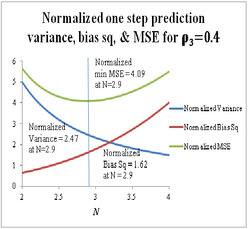
where the first term on the right of the equal sign is the normalized 2nd order one-step prediction variance and the second term is the normalized bias squared from acceleration. This MSE is plotted as a function of N in Figure 1 along with both the variance and bias squared.

Figure 1

Clearly, only integer order steps are possible in a non-recursive estimator. However, for use in approximating the tuned 2nd order KF, this MSE plot is stepped in tenths of a unit to show more precisely where the minimum occurs. The minimum MSE of 4.09 occurs at N = 2.9. The tuned KF can be approximated by sizing the process noise covariance in the KF such that the effective recursive data window—i.e., the Kalman filter memory—matches N = 2.9 in Figure 1 (i.e., [math]\displaystyle{ \alpha \approx 0.85 }[/math] and [math]\displaystyle{ \beta \approx 0.53 }[/math]), where [math]\displaystyle{ \alpha = \frac {4N-2} {N(N+1)} }[/math]and [math]\displaystyle{ \beta = \frac {6} {N(N+1)} }[/math]. This hints at the fallacy of using a 2nd order estimator on accelerating targets as described in. Comparing this with the filtered position in demonstrates that the minimum MSE is a function of the time [math]\displaystyle{ \tau }[/math] of the desired estimate.

FOE as a multiple-model estimator

The FOE can be viewed as a non-recursive multiple-model (MM) estimator composed of 2nd and 3rd order estimator models with the fraction [math]\displaystyle{ 0\le f_3 \le 1 }[/math] as the interpolation factor. Since the filtered position is generally used for comparisons in the literature, consider now the normalized MSE for the position estimate:

[math]\displaystyle{ MSE = \frac {1} {N}+\frac {3(N-1)} {N(N+1)}+ f_3^2\frac {5(N-1)(N-2)}{N ((N+1)(N+2)}+\rho_3^2 \left [\frac {(N-1)(N-2)}{6}\right ] ^2 (1-f_3)^2 }[/math]

Note that this differs from the one-step prediction MSE in that the signs within the parentheses containing N are reversed. The higher order pattern continues here also. Normalized with respect to the measurement noise variance, the minimum position MSE reduces for equally spaced samples to

[math]\displaystyle{ MSE_{min} = \frac {4N-2} {N(N+1)}+ f_{3,opt}\frac {5(N-1)(N-2)}{N ((N+1)(N+2)} }[/math]

where [math]\displaystyle{ |\upsilon_3|^2=\frac {180}{N(N^2-1)(N^2-4)} }[/math]

in [math]\displaystyle{ f_{3,opt}= \frac {\rho_3^2} {\rho_3^2+|\upsilon_3|^2} }[/math]

Figure 2

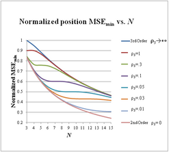
A plot of the position [math]\displaystyle{ MSE_{min} }[/math] as a function of N for various values of [math]\displaystyle{ \rho_3 }[/math] is shown in Figure 2, where there are several points of interest: First, the 2nd and 3rd order MSEs track each other very closely and bound all the [math]\displaystyle{ MSE_{min} }[/math] (interpolated) curves. Second, the curves drop rapidly to a knee. Third, the [math]\displaystyle{ MSE_{min} }[/math] curves flatten out beyond the knee yielding virtually no increase in accuracy until they begin to approach the 3rd order MSE (variance). This suggests that choosing a window at the knee of the curve is advantageous—to be demonstrated below.

Figure 3

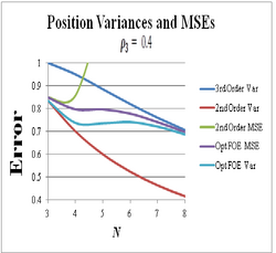
Consider again the scenario of, in this case as the target maneuvers. After traveling at a constant velocity, the target accelerates at [math]\displaystyle{ 20 m/s^2 }[/math] for 20 seconds and then continues again at a constant velocity. At worst case acceleration, [math]\displaystyle{ \rho_3= 0.4 }[/math]. The [math]\displaystyle{ MSE_{min} }[/math] is plotted in Figure 3 of as a function of N. Also shown are the 2nd order MSE as well as the 2nd and 3rd order MSEs (variances only since the bias is zero in each case) similar to those in Figure 2. There is a fifth curve not previously addressed: the variance portion of the optimal MSE. The variance also levels off for several increments of N like the [math]\displaystyle{ MSE_{min} }[/math]. Both the variance and [math]\displaystyle{ MSE_{min} }[/math] approach the 3rd order variance as [math]\displaystyle{ N \to \infty }[/math].

As the acceleration varies from zero to maximum, the MSE is automatically adjusted (no external tinkering or adaptivity) between the variance at [math]\displaystyle{ \rho_3 = 0 }[/math] and maximum [math]\displaystyle{ MSE_{min} }[/math] at [math]\displaystyle{ \rho_3 = 0.4 }[/math]. In other words, the MSE rides up and down the quadratic curve of the variance plus bias squared as a function of changes in acceleration [math]\displaystyle{ \rho_3 }[/math] for any given value of N in the position estimate:

[math]\displaystyle{ MSE = \frac {4N-2} {N(N+1)}+ \rho_3^2 \left [\frac {(N-1)(N-2)}{6}\right ]^2 }[/math]

Figure 4

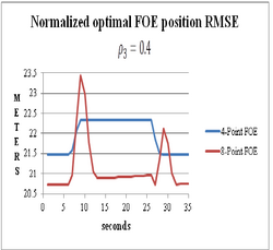
Choosing N = 4 at the knee of the [math]\displaystyle{ MSE_{min} }[/math] curve in Figure 3 yields the RMSE (square root of the MSE, which is more often used for comparison in the literature) shown in Figure 4. On the other hand, choosing N = 8 yields the second curve in Figure 4. As shown in Figure 3, the optimal 8–point FOE is essentially a 3rd order non-recursive estimator which yields less than 4% RMSE improvement over the optimal 4-point FOE in the case of no acceleration. However, in the case of maximum acceleration the optimal 8-point MSE is markedly volatile and has large error spikes that can confuse a tracker, one spike exceeding the optimal 4-point MSE for worst case acceleration by more than the optimal 4-point MSE exceeds the optimal 8-point MSE in the absence of acceleration. Obviously, higher values of N produce larger error spikes.

Since trackers encounter greatest difficulties and often lose track during target maneuvers at maximum acceleration, the much smoother [math]\displaystyle{ MSE_{min} }[/math]transition of the optimal 4-point FOE has a major advantage over larger data windows.

IMM compared with the optimal FOE

The 4-point FOE in Figure 4 yields much smoother MSE transitions than the IMM (as well as the KF) in the parallel 1 Hz case of. It produces no error spikes or volatility as do the 8-point FOE and the IMM. In this example only 4 multiplies, 3 adds, and a window shift are required to implement the 4-point FOE, significantly few operations than required by the IMM or KF. Similar comparisons of several additional MMs from the literature with the optimal FOE are made in

Of the KF based MMs, the interacting MM (IMM) is generally considered the state-of-the-art tracking model and usually the method of choice. Since two model IMMs are most often used, consider the following two models: 2nd and 3rd order KFs. The estimated IMM state equation is the sum of the 2nd order KF times the model probability [math]\displaystyle{ \mu_1(k) }[/math] plus the 3rd order KF times the model probability [math]\displaystyle{ \mu_2(k) }[/math]:

[math]\displaystyle{ \hat X(k|k) = \hat X_1(k|k)\mu_1(k)+\hat X_2 (k|k)\mu_2(k) }[/math]

where [math]\displaystyle{ \hat X_1(k|k) }[/math] represents the 2nd order KF, [math]\displaystyle{ \hat X_2 (|k|k) }[/math] represents the 3rd order KF, and k represents the time increment. Since the model probabilities sum to one, i.e., [math]\displaystyle{ \mu_1(k)+\mu_2(k)=1 }[/math]; this is actually linear interpolation, where [math]\displaystyle{ \mu_1(k) }[/math] is analogous to [math]\displaystyle{ (1 - f_3) }[/math] in the FOE and [math]\displaystyle{ \mu_2(k) }[/math] is analogous to [math]\displaystyle{ f_3 }[/math]. Therefore, this two model IMM is analogous to the optimal FOE in that it also interpolates between 2nd and 3rd order estimators. Two model IMM interpolation is formed during each recursive cycle involving the interactively produced model probabilities.

As in the case of the FOE, this suggests a more descriptive estimate equal to the sum of the 2nd order KF plus the difference between the 3rd and 2nd order KFs times [math]\displaystyle{ \mu_2(k) }[/math] :

[math]\displaystyle{ \hat X(k|k) = \hat X_1(k|k)+[\hat X_2 (k|k)-\hat X_1(k|k]\mu_2(k) }[/math]

In this formulation the difference between the 3rd and 2nd order KFs effectively augments the 2nd order KF with a fraction of the estimated target acceleration as a function of [math]\displaystyle{ \mu_2(k) }[/math]—as does [math]\displaystyle{ f_3 }[/math] in the FOE.

One major difference between the IMM and optimal FOE is that the IMM is not optimum. The IMM model probabilities and interpolation are based on likelihoods and ad hoc transition probabilities with no mechanism for minimizing the MSE. Of course, not being optimum at any time increment k, the IMM cannot achieve the optimal FOE accuracy shown in Figure 2.

Moveover, the IMM [math]\displaystyle{ \mu_2(k) }[/math] fails to meet the boundary condition of zero to implement the 2nd order estimator in the absence of acceleration, which the FOE [math]\displaystyle{ f_{3,opt} }[/math] does. This results from the fact that the likelihoods do not sum to unity even though the model probabilities do. This causes an IMM bias toward a non-existent acceleration and unnecessarily increases the MSE above the 2nd order variance. Another major difference between the IMM and FOE is that the IMM is adaptive whereas the FOE is not.

In order to make a reasonable comparison of the IMM with the FOE, reference constructs a non-recursive IMM analogy (IMMA). It includes [math]\displaystyle{ \mu_2(k) }[/math] which does go to zero allowing the 2nd order estimator to be implemented. Since the FOE is based on the actual acceleration not a noisy estimate, the acceleration estimate for the IMMA is assumed to be the expected value of the estimate, i.e., the actual acceleration. This is described here as the ideal for the purpose of illustration. These two modifications make the IMMA compatible for comparison with the FOE.

Figure 5

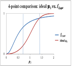
The [math]\displaystyle{ \mu_2(k) }[/math] based on the expected value or actual acceleration (described here as the ideal [math]\displaystyle{ \mu_2 }[/math] where the k is dropped) then varies between zero and one in an S-shaped curve as a function of [math]\displaystyle{ \rho_3 }[/math], as does [math]\displaystyle{ f_{3,opt} }[/math]. This is shown in Figure 5, where a 4-point data window is assumed.

Figure 6

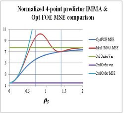
Two significant points of interest stand out as shown by the vertical lines. First, the largest deviation of the ideal [math]\displaystyle{ \mu_2 }[/math] from [math]\displaystyle{ f_{3,opt} }[/math] occurs near [math]\displaystyle{ \rho_3 = 0.7 }[/math]. Second, the two curves cross near [math]\displaystyle{ \rho_3 = 1.4 }[/math]. A comparison of the one-step predictor IMMA MSE as a function of ideal [math]\displaystyle{ \mu_2 }[/math] with the FOE [math]\displaystyle{ MSE_{min} }[/math] is given in Figure 6. For the IMMA, the linear interpolation factor [math]\displaystyle{ f_3 }[/math] is replaced in the normalized FOE MSE by the ideal [math]\displaystyle{ \mu_2 }[/math] as the interpolation factor for ideal IMMA MSE plotting.

Included in Figure 6 for reference are a curve of the 3rd order variance, 2nd order variance, and the 2nd order MSE. The large deviation of [math]\displaystyle{ \mu_2 }[/math] from [math]\displaystyle{ f_{3,opt} }[/math] in Figure 5 has a profound effect on the ideal IMMA MSE as shown in Figure 6. The ideal IMMA MSE exceeds the FOE MSE most near [math]\displaystyle{ \rho_3 = 0.7 }[/math], about where the [math]\displaystyle{ \mu_2 }[/math] differs most from [math]\displaystyle{ f_{3,opt} }[/math] in Figure 5. In addition, the ideal IMMA MSE exceeds the 3rd order variance most near [math]\displaystyle{ \rho_3 = 0.85 }[/math], even though the specific purpose of interpolation in the IMM is to produce an MSE smaller than the 3rd order variance. Nevertheless, as expected, the two MSE curves do osculate near [math]\displaystyle{ \rho_3 = 1.4 }[/math], where [math]\displaystyle{ \mu_2 }[/math] and [math]\displaystyle{ f_{3,opt} }[/math] cross in Figure 5.

Figure 7

Furthermore, the MSE is exacerbated in the non-ideal IMMA by adaptivity, as shown in Figure 7 where the IMMA from noisy [math]\displaystyle{ \mu_2 }[/math] is superimposed on the curves in Figure 6 (although there is a slight change in scale to accommodate the larger noisy IMMA MSE). Reference describes this in great detail. Clearly, since Figure 6 includes the ideal [math]\displaystyle{ \mu_2 }[/math] based on the expected value of acceleration, i.e., the actual acceleration; an estimate which includes measurement noise can only degrade the accuracy—as shown in Figure 7.

Indeed, not only is the noisy IMMA MSE larger than the 3rd order variance (by nearly a factor of two at the worst point), once the noisy IMMA MSE exceeds the 3rd order variance, it does not drop below as does the ideal IMMA. In contrast, the optimal FOE MSE (i.e., [math]\displaystyle{ MSE_{min} }[/math]) always remains less than the 3rd order variance.

This analysis compellingly suggests that adaptivity significantly degrades IMM accuracy rather than improving it. Of course, this should not come as a surprise since for [math]\displaystyle{ \rho_3\lt 0.5 }[/math] , the acceleration is buried in the noise; i.e., [math]\displaystyle{ (a\Delta^2)/\sigma_\eta \lt 1 }[/math] (a signal-to-noise ratio likeness of less than 0 dB).

These analyses reveal the incredible and disconcerting lack of tracking literature that addresses fundamentals (e.g., optimal IMM interpolation, [math]\displaystyle{ \mu_2 }[/math] boundary conditions, and acceleration-to-noise ratio) and comparisons with standard benchmarks (e.g.; 2nd order, 3rd order, or other optimal estimators).

Deficiencies and oversights in the Kalman filter

Comparisons of the KF with the derivation, analysis, design, and implementation of MFOE have uncovered a number of deficiencies and oversights in the KF that are overcome by the MFOE. They are reported and discussed in.

References

- ↑ Jump up to: 1.00 1.01 1.02 1.03 1.04 1.05 1.06 1.07 1.08 1.09 1.10 1.11 Bell, J. W., Simple Disambiguation Of Orthogonal Projection In Kalman’s filter Derivation, Proceedings of the International Conference on Radar Systems, Glasgow, UK. October, 2012.
- ↑ Jump up to: 2.00 2.01 2.02 2.03 2.04 2.05 2.06 2.07 2.08 2.09 2.10 2.11 2.12 Bell, J. W., A Simple Kalman Filter Alternative: The Multi-Fractional Order Estimator, IET-RSN, Vol. 7, Issue 8, October 2013.
- ↑ Jump up to: 3.0 3.1 Kalman, R. E., A New Approach to Linear Filtering and Prediction Problems, Journal of Basic Engineering, Vol. 82D, Mar. 1960.
- ↑ Jump up to: 4.0 4.1 4.2 4.3 Sorenson, H. W., Least-squares estimation: Gauss to Kalman, IEEE Spectrum, July, 1970.
- ↑ Radar tracker
- ↑ Jump up to: 6.0 6.1 6.2 Burkhardt, R., et.al., Titan Systems Corporation Atlantic Aerospace Division; Shipboard IRST Processing with Enhanced Discrimination Capability; Sponsor: Naval Surface Warfare Center, Dahlgren, VA; Contract #: N00178-98-C-3020; September 19, 2000 (p. 41).
- ↑ Blom, H. A. P., An efficient filter for abruptly changing systems, in Proceedings of the 23rd IEEE Conference on Decision and Control Las Vegas, NV, Dec. 1984, 656-658.
- ↑ Blom, H. A. P., and Bar-Shalom, Y., The interacting multiple model algorithm for systems with Markovian switching coefficients, IEEE Trans. Autom. Control, 1988, 33, pp. 780–783
- ↑ Bar-Shalom, Y. and Li, X. R., Estimation and Tracking : Principles, Techniques, and Software Artech House Radar Library, Boston, 1993.
- ↑ Mazor, E., Averbuch, A., Bar-Shalom, Y., Dayan, J., Interacting Multiple Model Methods in Target Tracking: A Survey; IEEE T-AES, Jan 1998
- ↑ Jump up to: 11.0 11.1 11.2 11.3 Bell, Jeff (2020-01-27) (in en). Ordinary Least Squares Revolutionized: Establishing the Vital Missing Empirically Determined Statistical Prediction Variance. Rochester, NY. doi:10.2139/ssrn.2573840. https://papers.ssrn.com/abstract=2573840.
- ↑ Jump up to: 12.0 12.1 12.2 Brookner, E., Tracking and Kalman Filtering Made Easy, Wiley, New York, 1998.
- ↑ Jump up to: 13.0 13.1 Kingsley, S. and Quegan, S., Understanding Radar Systems, McGraw-Hill, New York, 1992.
- ↑ Bell, Jeff (2020-01-28) (in en). A Simple and Pragmatic Approximation to the Normal Cumulative Probability Distribution. Rochester, NY. doi:10.2139/ssrn.2579686. https://papers.ssrn.com/abstract=2579686.
- ↑ Lau, Tak Kit and Lin, Kai-wun, Evolutionary Tuning of Sigma-Point Kalman Filters, Robotics and Automation (ICRA), 2011 IEEE International Conference on
- ↑ Bernt M. et al., A Tool for Kalman Filter Tuning, http://www.netegrate.com/index_files/Research%20Library/Catalogue/Quantitative%20Analysis/Kalman%20Filter/A%20Tool%20for%20Kalman%20Filter%20Tuning(Akesson,%20Jorgensen%20and%20Poulsen).pdf
- ↑ Jump up to: 17.0 17.1 17.2 Blair, W. D., Bar-Shalom, Y., Tracking Maneuvering Targets With Multiple Sensors: Does More Data Always Mean Better Estimates? IEEE T-AES Vol. 32, No.1, Jan. 1996.
- ↑ http://site.infowest.com/personal/j/jeffbell/The2ndOrderEstimatorFallacy.pdf[bare URL PDF]
- ↑ Jump up to: 19.0 19.1 http://site.infowest.com/personal/j/jeffbell/KalmanFilterTuning.pdf[bare URL PDF]
- ↑ Jump up to: 20.0 20.1 http://site.infowest.com/personal/j/jeffbell/NovelTechniques.pdf[bare URL PDF]
- ↑ Jump up to: 21.0 21.1 Yang, Chun, Blasch, Erik, Characteristic Errors of the IMM Algorithm under Three Maneuver Models for an Accelerating Target, Information Fusion, 2008 11th International Conference on
- ↑ Jump up to: 22.0 22.1 Gomes, J., An Overview on Target Tracking Using Multiple Model Methods, Masters Thesis, https://fenix.tecnico.ulisboa.pt/downloadFile/395137804053/thesis.pdf
- ↑ Jump up to: 23.0 23.1 http://isif.org/fusion/proceedings/fusion02CD/pdffiles/papers/T1D03.pdf[bare URL PDF]
- ↑ Jump up to: 24.0 24.1 Watson, G. A., and Blair, W. D., Interacting Acceleration Compensation Algorithm for Tracking Maneuvering Targets. IEEE T-AES. Vol. 31, No. 3 July 1995.
- ↑ Jump up to: 25.0 25.1 25.2 Pitre, Ryan, A Comparison of Multiple-Model Target Tracking Algorithms: University of New Orleans Theses and Dissertation,. December, 2004.
- ↑ "Archived copy". Archived from the original on 2015-09-06. https://web.archive.org/web/20150906040306/http://www.igidr.ac.in/susant/TEACHING/ETRICS1/p03.pdf. Retrieved 2015-04-02.
- ↑ Jump up to: 27.0 27.1 http://site.infowest.com/personal/j/jeffbell/WhyTheIMMisSubOptimum.pdf[bare URL PDF]
- ↑ http://site.infowest.com/personal/j/jeffbell/WhatPriceAdaptivity.pdf[bare URL PDF]
- ↑ http://site.infowest.com/personal/j/jeffbell/KalmanFilterDeficiencies.pdf[bare URL PDF]