Overlap–add method

In signal processing, the overlap–add method is an efficient way to evaluate the discrete convolution of a very long signal [math]\displaystyle{ x[n] }[/math] with a finite impulse response (FIR) filter [math]\displaystyle{ h[n] }[/math]:

[math]\displaystyle{ y[n] = x[n] * h[n] \ \triangleq\ \sum_{m=-\infty}^{\infty} h[m] \cdot x[n - m] = \sum_{m=1}^{M} h[m] \cdot x[n - m], }[/math]

(Eq.1)

where h[m] = 0 for m outside the region [1, M]. This article uses common abstract notations, such as [math]\displaystyle{ y(t) = x(t) * h(t), }[/math] or [math]\displaystyle{ y(t) = \mathcal{H}\{x(t)\}, }[/math] in which it is understood that the functions should be thought of in their totality, rather than at specific instants [math]\displaystyle{ t }[/math] (see Convolution).

Fig 1: A sequence of five plots depicts one cycle of the overlap-add convolution algorithm. The first plot is a long sequence of data to be processed with a lowpass FIR filter. The 2nd plot is one segment of the data to be processed in piecewise fashion. The 3rd plot is the filtered segment, including the filter rise and fall transients. The 4th plot indicates where the new data will be added with the result of previous segments. The 5th plot is the updated output stream. The FIR filter is a boxcar lowpass with M=16 samples, the length of the segments is L=100 samples and the overlap is 15 samples.

The concept is to divide the problem into multiple convolutions of h[n] with short segments of [math]\displaystyle{ x[n] }[/math]:

[math]\displaystyle{ x_k[n]\ \triangleq\ \begin{cases} x[n + kL], & n = 1, 2, \ldots, L\\ 0, & \text{otherwise}, \end{cases} }[/math]

where L is an arbitrary segment length. Then:

[math]\displaystyle{ x[n] = \sum_{k} x_k[n - kL],\, }[/math]

and y[n] can be written as a sum of short convolutions:

[math]\displaystyle{ \begin{align} y[n] = \left(\sum_{k} x_k[n - kL]\right) * h[n] &= \sum_{k} \left(x_k[n - kL] * h[n]\right)\\ &= \sum_{k} y_k[n - kL], \end{align} }[/math]

where the linear convolution [math]\displaystyle{ y_k[n]\ \triangleq\ x_k[n] * h[n]\, }[/math] is zero outside the region [1, L + M − 1]. And for any parameter [math]\displaystyle{ N \ge L + M - 1,\, }[/math] it is equivalent to the N-point circular convolution of [math]\displaystyle{ x_k[n]\, }[/math] with [math]\displaystyle{ h[n]\, }[/math] in the region [1, N].  The advantage is that the circular convolution can be computed more efficiently than linear convolution, according to the circular convolution theorem:

[math]\displaystyle{ y_k[n]\ =\ \scriptstyle \text{IDFT}_N \displaystyle (\ \scriptstyle \text{DFT}_N \displaystyle (x_k[n])\cdot\ \scriptstyle \text{DFT}_N \displaystyle (h[n])\ ), }[/math]

(Eq.2)

where:

• DFT_N and IDFT_N refer to the Discrete Fourier transform and its inverse, evaluated over N discrete points, and
• L is customarily chosen such that N = L+M-1 is an integer power-of-2, and the transforms are implemented with the FFT algorithm, for efficiency.

Pseudocode

The following is a pseudocode of the algorithm:

(Overlap-add algorithm for linear convolution)
h = FIR_filter
M = length(h)
Nx = length(x)
N = 8 × 2^ceiling( log2(M) )     (8 times the smallest power of two bigger than filter length M.  See next section for a slightly better choice.)
step_size = N - (M-1)  (L in the text above)
H = DFT(h, N)
position = 0
y(1 : Nx + M-1) = 0

while position + step_size ≤ Nx do
    y(position+(1:N)) = y(position+(1:N)) + IDFT(DFT(x(position+(1:step_size)), N) × H)
    position = position + step_size
end

Efficiency considerations

Fig 2: A graph of the values of N (an integer power of 2) that minimize the cost function [math]\displaystyle{ \tfrac{N\left(\log_2 N + 1\right)}{N - M + 1} }[/math]

When the DFT and IDFT are implemented by the FFT algorithm, the pseudocode above requires about N (log₂(N) + 1) complex multiplications for the FFT, product of arrays, and IFFT. Each iteration produces N-M+1 output samples, so the number of complex multiplications per output sample is about:

[math]\displaystyle{ \frac{N (\log_2(N) + 1)}{N-M+1}.\, }[/math]

(Eq.3)

For example, when M=201 and N=1024, Eq.3 equals 13.67, whereas direct evaluation of Eq.1 would require up to 201 complex multiplications per output sample, the worst case being when both x and h are complex-valued. Also note that for any given M, Eq.3 has a minimum with respect to N. Figure 2 is a graph of the values of N that minimize Eq.3 for a range of filter lengths (M).

Instead of Eq.1, we can also consider applying Eq.2 to a long sequence of length [math]\displaystyle{ N_x }[/math] samples. The total number of complex multiplications would be:

[math]\displaystyle{ N_x\cdot (\log_2(N_x) + 1). }[/math]

Comparatively, the number of complex multiplications required by the pseudocode algorithm is:

[math]\displaystyle{ N_x\cdot (\log_2(N) + 1)\cdot \frac{N}{N-M+1}. }[/math]

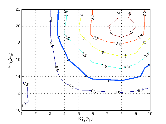
Hence the cost of the overlap–add method scales almost as [math]\displaystyle{ O\left(N_x\log_2 N\right) }[/math] while the cost of a single, large circular convolution is almost [math]\displaystyle{ O\left(N_x\log_2 N_x \right) }[/math]. The two methods are also compared in Figure 3, created by Matlab simulation. The contours are lines of constant ratio of the times it takes to perform both methods. When the overlap-add method is faster, the ratio exceeds 1, and ratios as high as 3 are seen.

Fig 3: Gain of the overlap-add method compared to a single, large circular convolution. The axes show values of signal length N_x and filter length N_h.

See also

• Overlap–save method

Further reading

• Oppenheim, Alan V.; Schafer, Ronald W. (1975). Digital signal processing. Englewood Cliffs, N.J.: Prentice-Hall. ISBN 0-13-214635-5. 
• Hayes, M. Horace (1999). Digital Signal Processing. Schaum's Outline Series. New York: McGraw Hill. ISBN 0-07-027389-8.

References

- ↑ Rabiner, Lawrence R.; Gold, Bernard (1975). "2.25". Theory and application of digital signal processing. Englewood Cliffs, N.J.: Prentice-Hall. pp. 63–65. ISBN 0-13-914101-4. https://archive.org/details/theoryapplicatio00rabi/page/63.