Partial Area Under the ROC Curve
The partial area under the ROC curve (pAUC) is a metric for the performance of a binary classifier.
It is computed based on the receiver operating characteristic (ROC) curve that illustrates the diagnostic ability of a given binary classifier system as its discrimination threshold is varied. The ROC curve is created by plotting the true positive rate (TPR) against the false positive rate (FPR) at various threshold settings.

The area under the ROC curve (AUC)[1][2] is often used to summarize in a single number the diagnostic ability of the classifier. The AUC is simply defined as the area of the ROC space that lies below the ROC curve.
However, in the ROC space there are regions where the values of FPR or TPR are unacceptable or not viable in practice. For instance, the region where FPR is greater than 0.8 involves that more than 80% of negative subjects are incorrectly classified as positives: this is unacceptable in many real cases. As a consequence, the AUC computed in the entire ROC space (i.e., with both FPR and TPR ranging from 0 to 1) can provide misleading indications.
To overcome this limitation of AUC, it was proposed[3] to compute the area under the ROC curve in the area of the ROC space that corresponds to interesting (i.e., practically viable or acceptable) values of FPR and TPR.
Basic concept
In the ROC space, where x=FPR (false positive rate) and y=ROC(x)=TPR (true positive rate), it is

The AUC is widely used, especially for comparing the performances of two (or more) binary classifiers: the classifier that achieves the highest AUC is deemed better. However, when comparing two classifiers and , three situations are possible:
- the ROC curve of is never above the ROC curve of
- the ROC curve of is never below the ROC curve of
- the classifiers’ ROC curves cross each other.
There is general consensus that in case 1 classifier is preferable and in case 2) classifier is preferable. Instead, in case 3) there are regions of the ROC space where is preferable and other regions where is preferable. This observation led to evaluating the accuracy of classifications by computing performance metrics that consider only a specific region of interest (RoI) in the ROC space, rather than the whole space. These performance metrics are commonly known as “partial AUC” (pAUC): the pAUC is the area of the selected region of the ROC space that lies under the ROC curve.
Partial AUC obtained by constraining FPR
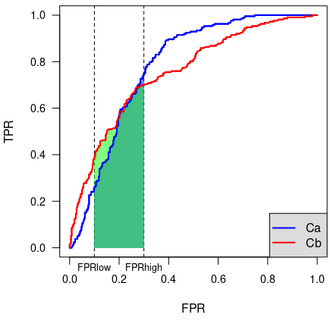
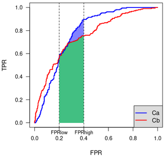
The idea of the partial AUC was originally proposed [3] with the goal of restricting the evaluation of given ROC curves in the range of false positive rates that are considered interesting for diagnostic purposes. Thus, the partial AUC was computed as the area under the ROC curve in the vertical band of the ROC space where FPR is in the range [, ].
 |
 |
|---|
The pAUC computed by constraining FPR helps compare two partial areas. Nonetheless, it has a few limitations:
- the RoI must be a vertical band of the ROC space;
- no criteria are given for identifying the RoI: it is expected that some expert is able to identify and ;
- when comparing two classifiers via the associated ROC curves, a relatively small change in selecting the RoI may lead to different conclusions: in the example above, considering the band where leads to conclude that is better, while considering the band where leads to conclude that is better.
Partial AUC obtained by constraining TPR
Another type of partial AUC is obtained by constraining the true positive rate, rather than the false positive rate. That is, the partial AUC is the area under the ROC curve and above the horizontal line .[4]
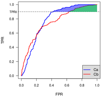
In other words, the pAUC is computed in the portion of the ROC space where the true positive rate is greater than a given threshold (no upper limit is used, since it would not make sense to limit the number of true positives).
This proposal too has a few limitations:
- by limiting the true positive rate, a limit on the false positive rate is also implicitly set;
- no criteria are given for identifying the RoI: it is expected that experts can identify the minimum acceptable true positive rate;
- when comparing two classifiers via the associated ROC curves, a relatively small change in selecting the RoI may lead to different conclusions: this happens when is close to the point where the given ROC curves cross each other.
Partial AUC obtained by constraining both FPR and TPR
A “two-way” pAUC was defined by constraining both the true positive and false negative rates.[5] A minimum value is specified for TPR and a maximum value is set for FPR, thus the RoI is the upper-left rectangle with vertices in points (, ), (, 1), (0, 1) and (0, ). The two-way pAUC is the area under the ROC curve that belongs to such rectangle.
The two-way pAUC is clearly more flexible than the pAUC defined by constraining only FPR or TPR. Actually, the latter two types of pAUC can be seen as special cases of the two-way pAUC.
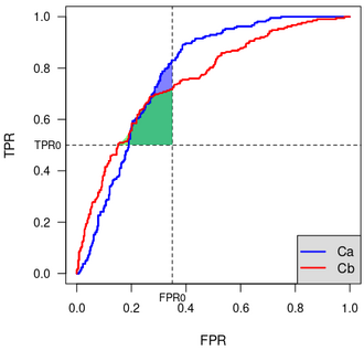
As with the pAUC described above, when comparing two classifiers via the associated ROC curves, a relatively small change in selecting the RoI may lead to different conclusions. This is a particularly delicate issue, since no criteria are given for identifying the RoI (as with the other mentioned pAUC, it is expected that experts can identify and ).
Partial AUC obtained by applying objective constraints to the region of interest
A few objective and sound criteria for defining the RoI were defined.[6][7] Specifically, the computation of pAUC can be restricted to the region where
- the considered classifiers are better (according to some performance metric of choice) than the random classification;
- the considered classifiers achieve at least a minimum value of some performance metrics of choice;
- the cost due to misclassifications by the considered classifiers is acceptable.
Defining the RoI based on the performance of the random classification
A possible way of defining the region where pAUC is computed consists of excluding the regions of the ROC space that represent performances worse than the performance achieved by the random classification.
Random classification evaluates a given item positive with probability and negative with probability (1-). In a dataset of n items, of which AP are actually positive, the best guess is obtained by setting ( is also known as the “prevalence” of the positives in the dataset).

It was shown that random classification with achieves , , and , on average.[6] Therefore, if the performance metrics of choice are TPR, FPR and precision, the RoI should be limited to the portion of the ROC space where , , and . It was shown that this region is the rectangle having vertices in (0,0), (0,1), (, 1), and (, ).[6]
This technique solves the problems of constraining TPR and FPR when two-ways pAUC has to be computed: .
The Ratio of Relevant Areas (RRA) indicator
Computing the pAUC requires that a RoI is first defined. For instance, when requiring better accuracy than mean random classification, the RoI is the rectangle having vertices in (0,0), (0,1), (, 1), and (, ). This implies that the size of the RoI varies depending on . Besides, the perfect ROC, i.e., the one that goes through point (0,1), has pAUC=(1-).
To get a pAUC-based indicator that accounts for and ranges in [0,1], RRA was proposed:[6]
RRA=1 indicates perfect accuracy, while RRA=0 indicates that the area under the ROC curve belonging to the RoI is null; thus accuracy is no better than random classification's.
Defining the RoI based on some performance metric threshold
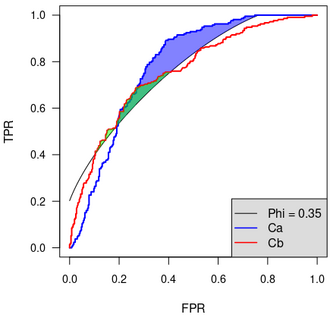
Several performance metrics are available for binary classifiers. One of the most popular is the Phi coefficient[8] (also known as the Matthews Correlation Coefficient[9]). Phi measures how better (or worse) is a classification, with respect to the random classification, which is characterized by Phi = 0. According to the reference values suggested by Cohen,[8] one can take Phi = 0.35 as a minimum acceptable level of Phi for a classification. In the ROC space, Phi equal to a non null constant corresponds to the arc of an ellipse, while Phi = 0 corresponds to the diagonal, i.e., to the points where FPR=TPR. So, considering the portion of the ROC where Phi>0.35 corresponds to defining the RoI as the portion of the ROC space above the ellipse. The pAUC is the area above the ellipse and under the ROC curve.
Defining the RoI based on the cost of misclassifications
Most binary classifiers yield misclassifications, which result in some cost.
The cost C of misclassifications is defined as , where is the unitary cost of a false negative, is the unitary cost of a false positive, and FN and FP are, respectively, the number of false negatives and false positives.
The normalized cost NC[10] is defined as .
By setting , we get
The average NC obtained via random classification is [6]
To evaluate a classifier excluding the performances whose cost is greater than , it is possible to define the RoI where the normalized cost is lower than the : such region is above the line

It is also possible to define the RoI where NC is less than a fraction of . In such case, the lower boundary of the RoI is the line
Different values of define the RoI in the same way as some of the best known performance metrics:
- equates to using FPR for delimiting the RoI
- equates to using precision for delimiting the RoI
- equates to using the F-1 score [11] for delimiting the RoI
- equates to using TPR for delimiting the RoI
Therefore, choosing a performance metric equates to choosing a specific value of the relative cost of false positives with respect to false negatives. In the ROC space, the slope of the line that represents constant normalized cost (hence, constant total cost) depends on , or, equivalently, on the performance metrics being used.
It is common practice[12][13] to select as the best classification the point of the ROC curve with the highest value of Youden's J =TPR−FPR.[14] When considering the cost associated with the misclassifications, this practice corresponds to making a hypothesis on the relative cost of false positives and false negatives, which is rarely correct.[7]
How to compute pAUC and RRA
Software libraries to compute pAUC and RRA are available for Python and R.[15]
References
- ↑ Van der Schouw, Y.T.; Verbeek, A.; Ruijs, J.H. (1992). "ROC Curves For the Initial Assessment of New Diagnostic Tests". Family Practice 9 (4): 506–511. doi:10.1093/fampra/9.4.506. ISSN 0263-2136. PMID 1490547. http://dx.doi.org/10.1093/fampra/9.4.506.
- ↑ Bradley, Andrew P. (1997). "The use of the area under the ROC curve in the evaluation of machine learning algorithms" (in en). Pattern Recognition 30 (7): 1145–1159. doi:10.1016/S0031-3203(96)00142-2. ISSN 0031-3203. Bibcode: 1997PatRe..30.1145B. https://www.sciencedirect.com/science/article/pii/S0031320396001422.
- ↑ 3.0 3.1 McClish, D. K. (1989). "Analyzing a portion of the ROC curve". Medical Decision Making 9 (3): 190–195. doi:10.1177/0272989X8900900307. ISSN 0272-989X. PMID 2668680.
- ↑ Jiang, Y; Metz, C E; Nishikawa, R M (1996). "A receiver operating characteristic partial area index for highly sensitive diagnostic tests.". Radiology 201 (3): 745–750. doi:10.1148/radiology.201.3.8939225. ISSN 0033-8419. PMID 8939225. http://dx.doi.org/10.1148/radiology.201.3.8939225.
- ↑ Yang, Hanfang; Lu, Kun; Lyu, Xiang; Hu, Feifang (2017-07-14). "Two-way partial AUC and its properties". Statistical Methods in Medical Research 28 (1): 184–195. doi:10.1177/0962280217718866. ISSN 0962-2802. PMID 28707503. http://dx.doi.org/10.1177/0962280217718866.
- ↑ 6.0 6.1 6.2 6.3 6.4 Morasca, Sandro; Lavazza, Luigi (2020-08-19). "On the assessment of software defect prediction models via ROC curves". Empirical Software Engineering 25 (5): 3977–4019. doi:10.1007/s10664-020-09861-4. ISSN 1382-3256.
- ↑ 7.0 7.1 Lavazza, Luigi; Morasca, Sandro (2021-12-20). "Considerations on the region of interest in the ROC space". Statistical Methods in Medical Research 31 (3): 419–437. doi:10.1177/09622802211060515. ISSN 0962-2802. PMID 34928729. http://dx.doi.org/10.1177/09622802211060515.
- ↑ 8.0 8.1 Cohen, Jacob (1988). Statistical power analysis for the behavioral sciences, 2nd edition. Lawrence Earlbaum Associates. ISBN 9780203771587.
- ↑ Matthews, B.W. (1975). "Comparison of the predicted and observed secondary structure of T4 phage lysozyme". Biochimica et Biophysica Acta (BBA) - Protein Structure 405 (2): 442–451. doi:10.1016/0005-2795(75)90109-9. ISSN 0005-2795. PMID 1180967. http://dx.doi.org/10.1016/0005-2795(75)90109-9.
- ↑ Cahill, Jaspar; Hogan, James M.; Thomas, Richard (2013). "Predicting Fault-Prone Software Modules with Rank Sum Classification". 2013 22nd Australian Software Engineering Conference. IEEE. pp. 211–219. doi:10.1109/aswec.2013.33. ISBN 978-0-7695-4995-8. http://dx.doi.org/10.1109/aswec.2013.33.
- ↑ van Rijsbergen, C.J. (1979). Information Retrieval. Butterworth.
- ↑ Perkins, N.J.; Schisterman, E.F. (2006). "The inconsistency of "optimal" cutpoints obtained using two criteria based on the receiver operating characteristic curve". American Journal of Epidemiology 163 (7): 670–675. doi:10.1093/aje/kwj063. PMID 16410346.
- ↑ Akobeng, A.K. (2007). "Understanding diagnostic tests: Receiver operating characteristic curves". Acta Paediatrica 95 (5): 644–647. doi:10.1111/j.1651-2227.2006.00178.x. PMID 17376185.
- ↑ Youden, W. J. (1950). "Index for rating diagnostic tests". Cancer 3 (1): 32–35. doi:10.1002/1097-0142(1950)3:1<32::aid-cncr2820030106>3.0.co;2-3. ISSN 0008-543X. PMID 15405679.
- ↑ Python Library Download, R Library Download at the website of the University of Insubria. A brief description of the libraries is also available.
 |
