Period-doubling bifurcation

In dynamical systems theory, a period-doubling bifurcation occurs when a slight change in a system's parameters causes a new periodic trajectory to emerge from an existing periodic trajectory—the new one having double the period of the original. With the doubled period, it takes twice as long (or, in a discrete dynamical system, twice as many iterations) for the numerical values visited by the system to repeat themselves. A period-halving bifurcation occurs when a system switches to a new behavior with half the period of the original system.

A period-doubling cascade is an infinite sequence of period-doubling bifurcations. Such cascades are a common route by which dynamical systems develop chaos. In hydrodynamics, they are one of the possible routes to turbulence.

Period-halving bifurcations (L) leading to order, followed by period-doubling bifurcations (R) leading to chaos.

Examples

Bifurcation diagram for the logistic map. It shows the attractor values, like [math]\displaystyle{ x_* }[/math] and [math]\displaystyle{ x'_* }[/math], as a function of the parameter [math]\displaystyle{ r }[/math].

Logistic map

The logistic map is

[math]\displaystyle{ x_{n+1} = r x_n (1 - x_n) }[/math]

where [math]\displaystyle{ x_n }[/math] is a function of the (discrete) time [math]\displaystyle{ n = 0, 1, 2, \ldots }[/math]. The parameter [math]\displaystyle{ r }[/math] is assumed to lie in the interval [math]\displaystyle{ [0,4] }[/math], in which case [math]\displaystyle{ x_n }[/math] is bounded on [math]\displaystyle{ [0,1] }[/math].

For [math]\displaystyle{ r }[/math] between 1 and 3, [math]\displaystyle{ x_n }[/math] converges to the stable fixed point [math]\displaystyle{ x_* = (r-1)/r }[/math]. Then, for [math]\displaystyle{ r }[/math] between 3 and 3.44949, [math]\displaystyle{ x_n }[/math] converges to a permanent oscillation between two values [math]\displaystyle{ x_* }[/math] and [math]\displaystyle{ x'_* }[/math] that depend on [math]\displaystyle{ r }[/math]. As [math]\displaystyle{ r }[/math] grows larger, oscillations between 4 values, then 8, 16, 32, etc. appear. These period doublings culminate at [math]\displaystyle{ r \approx 3.56995 }[/math], beyond which more complex regimes appear. As [math]\displaystyle{ r }[/math] increases, there are some intervals where most starting values will converge to one or a small number of stable oscillations, such as near [math]\displaystyle{ r=3.83 }[/math].

In the interval where the period is [math]\displaystyle{ 2^n }[/math] for some positive integer [math]\displaystyle{ n }[/math], not all the points actually have period [math]\displaystyle{ 2^n }[/math]. These are single points, rather than intervals. These points are said to be in unstable orbits, since nearby points do not approach the same orbit as them.

quadratic map

Real version of complex quadratic map is related with real slice of the Mandelbrot set.

• 

  Period-doubling cascade in an exponential mapping of the Mandelbrot set

• 

  1D version with an exponential mapping

• 

  period doubling bifurcation

Kuramoto–Sivashinsky equation

Period doubling in the Kuramoto–Sivashinsky equation with periodic boundary conditions. The curves depict solutions of the Kuramoto–Sivashinsky equation projected onto the energy phase plane (E, dE/dt), where E is the L²-norm of the solution. For ν = 0.056, there exists a periodic orbit with period T ≈ 1.1759. Near ν ≈ 0.0558, this solution splits into 2 orbits, which further separate as ν is decreased. Exactly at the transitional value of ν, the new orbit (red-dashed) has double the period of the original. (However, as ν increases further, the ratio of periods deviates from exactly 2.)

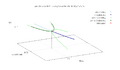
The Kuramoto–Sivashinsky equation is an example of a spatiotemporally continuous dynamical system that exhibits period doubling. It is one of the most well-studied nonlinear partial differential equations, originally introduced as a model of flame front propagation.

The one-dimensional Kuramoto–Sivashinsky equation is

[math]\displaystyle{ u_t + u u_x + u_{xx} + \nu \, u_{xxxx} = 0 }[/math]

A common choice for boundary conditions is spatial periodicity: [math]\displaystyle{ u(x + 2 \pi, t) = u(x,t) }[/math].

For large values of [math]\displaystyle{ \nu }[/math], [math]\displaystyle{ u(x,t) }[/math] evolves toward steady (time-independent) solutions or simple periodic orbits. As [math]\displaystyle{ \nu }[/math] is decreased, the dynamics eventually develops chaos. The transition from order to chaos occurs via a cascade of period-doubling bifurcations, one of which is illustrated in the figure.

Logistic map for a modified Phillips curve

Consider the following logistical map for a modified Phillips curve:

[math]\displaystyle{ \pi_{t} = f(u_{t}) + b \pi_{t}^e }[/math]

[math]\displaystyle{ \pi_{t+1} = \pi_{t}^e + c (\pi_{t} - \pi_{t}^e) }[/math]

[math]\displaystyle{ f(u) = \beta_{1} + \beta_{2} e^{-u} \, }[/math]

[math]\displaystyle{ b \gt 0, 0 \leq c \leq 1, \frac {df} {du} \lt 0 }[/math]

where :

• [math]\displaystyle{ \pi }[/math] is the actual inflation
• [math]\displaystyle{ \pi^e }[/math] is the expected inflation,
• u is the level of unemployment,
• [math]\displaystyle{ m - \pi }[/math] is the money supply growth rate.

Keeping [math]\displaystyle{ \beta_{1} = -2.5, \ \beta_{2} = 20, \ c = 0.75 }[/math] and varying [math]\displaystyle{ b }[/math], the system undergoes period-doubling bifurcations and ultimately becomes chaotic.

Experimental observation

Period doubling has been observed in a number of experimental systems. There is also experimental evidence of period-doubling cascades. For example, sequences of 4 period doublings have been observed in the dynamics of convection rolls in water and mercury. Similarly, 4-5 doublings have been observed in certain nonlinear electronic circuits. However, the experimental precision required to detect the i^th doubling event in a cascade increases exponentially with i, making it difficult to observe more than 5 doubling events in a cascade.

See also

• List of chaotic maps
• Complex quadratic map
• Feigenbaum constants
• Universality (dynamical systems)
• Sharkovskii's theorem

References

• Alligood, Kathleen T.; Sauer, Tim; Yorke, James (1996). Chaos: An Introduction to Dynamical Systems. Textbooks in Mathematical Sciences. Springer-Verlag New York. doi:10.1007/0-387-22492-0_3. ISBN 978-0-387-94677-1. 
• Giglio, Marzio; Musazzi, Sergio; Perini, Umberto (1981). "Transition to Chaotic Behavior via a Reproducible Sequence of Period-Doubling Bifurcations". Physical Review Letters 47 (4): 243–246. doi:10.1103/PhysRevLett.47.243. ISSN 0031-9007. Bibcode: 1981PhRvL..47..243G. 
• Kalogirou, A.; Keaveny, E. E.; Papageorgiou, D. T. (2015). "An in-depth numerical study of the two-dimensional Kuramoto–Sivashinsky equation". Proceedings of the Royal Society A: Mathematical, Physical and Engineering Sciences 471 (2179): 20140932. doi:10.1098/rspa.2014.0932. ISSN 1364-5021. PMID 26345218. Bibcode: 2015RSPSA.47140932K. 
• Kuznetsov, Yuri A. (2004). Elements of Applied Bifurcation Theory. Applied Mathematical Sciences. 112 (3rd ed.). Springer-Verlag. ISBN 0-387-21906-4. 
• Libchaber, A.; Laroche, C.; Fauve, S. (1982). "Period doubling cascade in mercury, a quantitative measurement". Journal de Physique Lettres 43 (7): 211–216. doi:10.1051/jphyslet:01982004307021100. ISSN 0302-072X. https://hal.archives-ouvertes.fr/jpa-00232033/file/ajp-jphyslet_1982_43_7_211_0.pdf. 
• Papageorgiou, D.T.; Smyrlis, Y.S. (1991), "The route to chaos for the Kuramoto-Sivashinsky equation", Theoret. Comput. Fluid Dynamics 3: 15–42, doi:10.1007/BF00271514, ISSN 1432-2250, Bibcode: 1991ThCFD...3...15P 
• Smyrlis, Y. S.; Papageorgiou, D. T. (1991). "Predicting chaos for infinite dimensional dynamical systems: the Kuramoto-Sivashinsky equation, a case study.". Proceedings of the National Academy of Sciences 88 (24): 11129–11132. doi:10.1073/pnas.88.24.11129. ISSN 0027-8424. PMID 11607246. Bibcode: 1991PNAS...8811129S. 
• Strogatz, Steven (2015). Nonlinear Dynamics and Chaos: With applications to Physics, Biology, Chemistry and Engineering (2nd ed.). CRC Press. ISBN 978-0813349107. 
• Cheung, P. Y.; Wong, A. Y. (1987). "Chaotic behavior and period doubling in plasmas". Physical Review Letters 59 (5): 551–554. doi:10.1103/PhysRevLett.59.551. ISSN 0031-9007. PMID 10035803. Bibcode: 1987PhRvL..59..551C. 

External links

• Connecting period-doubling cascades to chaos