Physics:Blade element theory

Blade element theory (BET) is a mathematical process originally designed by William Froude (1878), David W. Taylor (1893) and Stefan Drzewiecki (1885) to determine the behavior of propellers. It involves breaking a blade down into several small parts then determining the forces on each of these small blade elements. These forces are then integrated along the entire blade and over one rotor revolution in order to obtain the forces and moments produced by the entire propeller or rotor. One of the key difficulties lies in modelling the induced velocity on the rotor disk. Because of this the blade element theory is often combined with momentum theory to provide additional relationships necessary to describe the induced velocity on the rotor disk, producing blade element momentum theory. At the most basic level of approximation a uniform induced velocity on the disk is assumed:

[math]\displaystyle{ v_i = \sqrt{\frac{T}{A} \cdot \frac{1}{2 \rho}}. }[/math]

Alternatively the variation of the induced velocity along the radius can be modeled by breaking the blade down into small annuli and applying the conservation of mass, momentum and energy to every annulus. This approach is sometimes called the Froude–Finsterwalder equation.

If the blade element method is applied to helicopter rotors in forward flight it is necessary to consider the flapping motion of the blades as well as the longitudinal and lateral distribution of the induced velocity on the rotor disk. The most simple forward flight inflow models are first harmonic models.

Simple blade element theory

Fig 1. Blade element

Fig 2. Aerodynamic forces on a blade element.

While the momentum theory is useful for determining ideal efficiency, it gives a very incomplete account of the action of screw propellers, neglecting among other things the torque. In order to investigate propeller action in greater detail, the blades are considered as made up of a number of small elements, and the air forces on each element are calculated. Thus, while the momentum theory deals with the flow of the air, the blade-element theory deals primarily with the forces on the propeller blades. The idea of analyzing the forces on elementary strips of propeller blades was first published by William Froude in 1878. It was also worked out independently by Drzewiecki and given in a book on mechanical flight published in Russia seven years later, in 1885. Again, in 1907, Lanchester published a somewhat more advanced form of the blade-element theory without knowledge of previous work on the subject. The simple blade-element theory is usually referred to, however, as the Drzewiecki theory, for it was Drzewiecki who put it into practical form and brought it into general use. Also, he was the first to sum up the forces on the blade elements to obtain the thrust and torque for a whole propeller and the first to introduce the idea of using airfoil data to find the forces on the blade elements.

In the Drzewiecki blade-element theory the propeller is considered a warped or twisted airfoil, each segment of which follows a helical path and is treated as a segment of an ordinary wing. It is usually assumed in the simple theory that airfoil coefficients obtained from wind tunnel tests of model wings (ordinarily tested with an aspect ratio of 6) apply directly to propeller blade elements of the same cross-sectional shape.

The air flow around each element is considered two-dimensional and therefore unaffected by the adjacent parts of the blade. The independence of the blade elements at any given radius with respect to the neighbouring elements has been established theoretically and has also been shown to be substantially true for the working sections of the blade by special experiments made for the purpose. It is also assumed that the air passes through the propeller with no radial flow (i.e., there is no contraction of the slipstream in passing through the propeller disc) and that there is no blade interference.

Aerodynamic forces on a blade element

Consider the element at radius r, shown in Fig. 1, which has the infinitesimal length dr and the width b. The motion of the element in an aircraft propeller in flight is along a helical path determined by the forward velocity V of the aircraft and the tangential velocity 2πrn of the element in the plane of the propeller disc, where n represents the revolutions per unit time. The velocity of the element with respect to the air Vr is then the resultant of the forward and tangential velocities, as shown in Fig. 2. Call the angle between the direction of motion of the element and the plane of rotation Φ, and the blade angle β. The angle of attack α of the element relative to the air is then [math]\displaystyle{ \alpha=\beta-\phi }[/math].

Applying ordinary airfoil coefficients, the lift force on the element is:

[math]\displaystyle{ dL = \frac{1}{2}V_r^2 C_L b \, dr. }[/math]

Let γ be the angle between the lift component and the resultant force, or [math]\displaystyle{ \gamma=\arctan\frac{D}{L} }[/math]. Then the total resultant air force on the element is: [math]\displaystyle{ dR=\frac{\frac{1}{2}V_r^2 C_L b \, dr}{\cos\gamma}. }[/math]

The thrust of the element is the component of the resultant force in the direction of the propeller axis (Fig. 2), or [math]\displaystyle{ \begin{align} dT & = dR\cos(\phi+\gamma) \\ & = \frac{\frac{1}{2}V_r^2C_L b\cos(\phi+\gamma)}{\cos\gamma} dr, \end{align} }[/math] and since [math]\displaystyle{ V_r=\frac{V}{\sin\phi} }[/math] [math]\displaystyle{ dT = \frac{\frac{1}{2}V^2 C_L b\cos(\phi+\gamma)}{\sin^2\phi\cos\gamma} dr. }[/math]

For convenience let [math]\displaystyle{ K=\frac{C_Lb}{\sin^2\phi\cos\gamma} }[/math] and [math]\displaystyle{ T_c=K\cos(\phi+\gamma). }[/math]

Then [math]\displaystyle{ dT = \frac{1}{2}\rho V^2 T_c \, dr, }[/math] and the total thrust for the propeller (of B blades) is: [math]\displaystyle{ T=\frac{1}{2}\rho V^2B\int_{0}^{R} T_c \, dr. }[/math]

Referring again to Fig. 2, the tangential or torque force is

[math]\displaystyle{ dF=dR\sin(\phi+\gamma), }[/math]

and the torque on the element is

[math]\displaystyle{ dQ = r \, dR \, \sin(\phi+\gamma), }[/math]

which, if [math]\displaystyle{ Q_c=Kr\sin(\phi+\gamma) }[/math], can be written

[math]\displaystyle{ dQ=\frac{1}{2}\rho V^2 Q_c dr. }[/math]

The expression for the torque of the whole propeller is therefore

[math]\displaystyle{ Q = \frac{1}{2}\rho V^2 B\int_{0}^{R} Q_c dr. }[/math]

The horsepower absorbed by the propeller, or the torque horse-power, is

[math]\displaystyle{ QHP=\frac{2\pi nQ}{550} }[/math]

and the efficiency is

[math]\displaystyle{ \eta=\frac{THP}{QHP}=\frac{TV}{2\pi nQ}. }[/math]

Efficiency

Fig 3. Diagram of efficiency

Because of the variation of the blade width, angle, and airfoil section along the blade, it is not possible to obtain a simple expression for the thrust, torque, and efficiency of propellers in general. A single element at about two-thirds or three-fourths of the tip radius is, however, fairly representative of the whole propeller, and it is therefore interesting to examine the expression for the efficiency of a single element. The efficiency of an element is the ratio of the useful power to the power absorbed, or

[math]\displaystyle{ \begin{align} \eta & = \frac{dTV}{dQ2\pi n} \\ & = \frac{dR\cos(\phi+\gamma)V}{dR\sin(\phi+\gamma)2\pi nr} \\ & = \frac{\tan\phi}{\tan(\phi+\gamma)}. \end{align} }[/math]

Now tan Φ is the ratio of the forward to the tangential velocity, and [math]\displaystyle{ \tan\gamma=\frac{D}{L} }[/math]. According to the simple blade-element theory, therefore, the efficiency of an element of a propeller depends only on the ratio of the forward to the tangential velocity and on the [math]\displaystyle{ \frac{D}{L} }[/math] of the airfoil section.

The value of Φ which gives the maximum efficiency for an element, as found by differentiating the efficiency with respect to Φ and equating the result to zero, is

Fig 4. Airflow

[math]\displaystyle{ \phi=45^\circ-\frac{\gamma}{2} }[/math]

Fig 5. Multiplane with negative stagger

The variation of efficiency with 0 is shown in Fig. 3 for two extreme values of γ. The efficiency rises to a maximum at [math]\displaystyle{ 45^\circ-\frac{\gamma}{2} }[/math] and then falls to zero again at [math]\displaystyle{ 90^\circ-\gamma }[/math]. With an [math]\displaystyle{ \frac{L}{D} }[/math] of 28.6 the maximum possible efficiency of an element according to the simple theory is 0.932, while with an [math]\displaystyle{ \frac{L}{D} }[/math] of 9.5 it is only 0.812. At the values of Φ at which the most important elements of the majority of propellers work (10° to 15°) the effect of [math]\displaystyle{ \frac{L}{D} }[/math] on efficiency is still greater. Within the range of 10° to 15°, the curves in Fig. 3 indicate that it is advantageous to have both the [math]\displaystyle{ \frac{L}{D} }[/math] of the airfoil sections and the angle Φ (or the advance per revolution, and consequently the pitch) as high as possible.

Limitations

According to momentum theory, a velocity is imparted to the air passing through the propeller, and half of this velocity is given the air by the time it reaches the propeller plane. This increase of velocity of the air as it passes into the propeller disc is called the inflow velocity. It is always found where there is pressure discontinuity in a fluid. In the case of a wing moving horizontally, the air is given a downward velocity, as shown in Fig. 4., and theoretically half of this velocity is imparted in front of and above the wing, and the other half below and behind.

This induced downflow is present in the model wing tests from which the airfoil coefficients used in the blade-element theory are obtained; the inflow indicated by the momentum theory is therefore automatically taken into account in the simple blade-element theory. However, the induced downflow is widely different for different aspect ratios, being zero for infinite aspect ratio. Most model airfoil tests are made with rectangular wings having an arbitrarily chosen aspect ratio of 6, and there is no reason to suppose that the downflow in such a test corresponds to the inflow for each element of a propeller blade. In fact, the general conclusion drawn from an exhaustive series of tests, in which the pressure distribution was measured over 12 sections of a model propeller running in a wind tunnel, is that the lift coefficient of the propeller blade element differs considerably from that measured at the same angle of attack on an airfoil of aspect ratio 6. This is one of the greatest weaknesses of the simple blade-element theory.

Another weakness is that the interference between the propeller blades is not considered. The elements of the blades at any particular radius form a cascade similar to a multiplane with negative stagger, as shown in Fig. 4. Near the tips where the gap is large the interference is very small, but in toward the blade roots it is quite large.

In actual propellers there is a tip loss which the blade-element theory does not take into consideration. The thrust and torque forces as computed by means of the theory are therefore greater for the elements near the tip than those found by experiment.

In order to eliminate scale effect, the wind tunnel tests on model wings should be run at the same value of Reynolds number (scale) as the corresponding elements in the propeller blades. Airfoil characteristics measured at such a low scale as, for example, an air velocity of 30 m.p.h. with a 3-in. chord airfoil, show peculiarities not found when the tests are run at a scale comparable with that of propeller elements. The standard propeller section characteristics given in Figs. 11, 12, 13, and 14 were obtained from high Reynolds-number tests in the Variable Density Tunnel of the N.A.C.A., and, fortunately, for all excepting the thickest of these sections there is very little difference in characteristics at high and low Reynolds numbers. These values may be used with reasonable accuracy as to scale for propellers operating at tip speeds well below the speed of sound in air, and therefore relatively free from any effects of compressibility.

The poor accuracy of the simple blade-element theory is very well shown in a report by Durand and Lesley, in which they have computed the performance of a large number of model propellers (80) and compared the computed values with the actual performances obtained from tests on the model propellers themselves. In the words of the authors:

The divergencies between the two sets of results, while showing certain elements of consistency, are on the whole too large and too capriciously distributed to justify the use of the theory in this simplest form for other than approximate estimates or for comparative purposes.

The airfoils were tested in two different wind tunnels and in one of the tunnels at two different air velocities, and the propeller characteristics computed from the three sets of airfoil data differ by as much as 28%, illustrating quite forcibly the necessity for having the airfoil tests made at the correct scale.

In spite of all its inaccuracies the simple blade-element theory has been a useful tool in the hands of experienced propeller designers. With it a skilful designer having a knowledge of suitable empirical factors can design propellers which usually fit the main conditions imposed upon them fairly well in that they absorb the engine power at very nearly the proper revolution speed. They are not, however, necessarily the most efficient propellers for their purpose, for the simple theory is not sufficiently accurate to show slight differences in efficiency due to changes in pitch distribution, plan forms, etc.

Example

Fig 6. Ordinates of standard propeller section based on R.A.F.-6.

In choosing a propeller to analyze, it is desirable that its aerodynamic characteristics be known so that the accuracy of the calculated results can be checked. It is also desirable that the analysis be made of a propeller operating at a relatively low tip speed in order to be free from any effects of compressibility and that it be running free from body interference. The only propeller tests which satisfy all of these conditions are tests of model propellers in a wind tunnel. We shall therefore take for our example the central or master propeller of a series of model wood propellers of standard Navy form, tested by Dr. W. F. Durand at Stanford University. This is a two-bladed propeller 3 ft. in diameter, with a uniform geometrical pitch of 2.1 ft. (or a pitch-diameter ratio of 0.7). The blades have standard propeller sections based on the R.A.F-6 airfoil (Fig. 6), and the blade widths, thicknesses, and angles are as given in the first part of Table I. In our analysis we shall consider the propeller as advancing with a velocity of 40 m.p.h. and turning at the rate of 1,800 r.p.m.

Fig 7. Two flat sections facing each other face-to-face.

For the section at 75% of the tip radius, the radius is 1.125 ft., the blade width is 0.198 ft., the thickness ratio is 0.107, the lower camber is zero, and the blade angle β is 16.6°.

The forward velocity [math]\displaystyle{ \begin{align} V &= 40\ \mathrm{m.p.h.}\\ & = \frac{40\times88}{60} \\ & = 58.65\ \text{ft./sec.}, \end{align} }[/math]

Fig 8. Correction to lift coefficient for the convex lower chamber. (NOTE: For a Section with Lower Chamber, [math]\displaystyle{ C_L=C_{L(flat face)} -\Delta C_L }[/math])

and [math]\displaystyle{ \begin{align} n & = \frac{1800}{60} \\ & = 30\ \text{r.p.s.} \end{align} }[/math]

The path angle

[math]\displaystyle{ \begin{align} \phi& = \arctan\frac{V}{2\pi rn} \\ & = \arctan\frac{58.65}{2\pi\times1.125\times30} \\ & = 15.5^\circ \end{align} }[/math]

The angle of attack is therefore

[math]\displaystyle{ \begin{align} \alpha & = \beta-\phi \\ & = 16.6^\circ-15.5^\circ \\ & = 1.1^\circ \\ \end{align} }[/math]

From Fig. 7, for a flat-faced section of thickness ratio 0.107 at an angle of attack of 1.1°, γ = 3.0°, and, from Fig. 9, C_L = 0.425. (For sections having lower camber, C_L should be corrected in accordance with the relation given in Fig. 8, and γ is given the same value as that for a flat-faced section having the upper camber only.)

Fig 9. Thrust and torque grading curves.

Then

[math]\displaystyle{ \begin{align} K & = \frac{C_Lb}{\sin^2\phi\cos\gamma} \\ & = \frac{0.425\times0.198}{0.2672^2\times0.999} \\ & = 1.180, \end{align} }[/math]

and,

[math]\displaystyle{ \begin{align} T_C & = K\cos(\phi+\gamma) \\ & = 1.180\times\cos18.5^\circ \\ & = 1.119. \\ \end{align} }[/math]

Also,

[math]\displaystyle{ \begin{align} Q_C & = Kr\sin(\phi+\gamma) \\ & = 1.180\times1.125\times\sin18.5^\circ \\ & = 1.421. \end{align} }[/math]

The computations of T_c and Q_c for six representative elements of the propeller are given in convenient tabular form in Table I, and the values of T_c and Q_c are plotted against radius in Fig. 9. The curves drawn through these points are sometimes referred to as the torque grading curves. The areas under the curve represent [math]\displaystyle{ \int_{0}^{R} T_c dr }[/math] and [math]\displaystyle{ \int_{0}^{R} Q_c dr, }[/math] these being the expressions for the total thrust and torque per blade per unit of dynamic pressure due to the velocity of advance. The areas may be found by means of a planimeter, proper consideration, of course, being given to the scales of values, or the integration may be performed approximately (but with satisfactory accuracy) by means of Simpson's rule.

In using Simpson's rule the radius is divided into an even number of equal parts, such as ten. The ordinate at each division can then be found from the grading curve. If the original blade elements divide the blade into an even number of equal parts it is not necessary to plot the grading curves, but the curves are advantageous in that they show graphically the distribution of thrust and torque along the blade. They also provide a check upon the computations, for incorrect points will not usually form a fair curve.

Table I. — Computations for Propeller Analysis with Simple Blade- element Theory

D = 3.0 ft. p = 2.1 ft.	Forward velocity = 40 m.p.h. = 58.65 ft. /sec. Rotational velocity = 1,800 r.p.m. = 30 r.p.s.
r/R	0.15	0.30	0.45	0.60	0.75	0.90
r (ft.)	0.225	0.450	0.675	0.900	1.125	1.350
b (ft.)	0.225	0.236	0.250	0.236	0.198	0.135
hv/b	0.190	0.200	0.167	0.133	0.107	0.090
hl/b	0.180	0.058	0.007	000	000	000
β(deg.)	56.1	36.6	26.4	20.4	16.6	13.9
2πrn	42.3	84.7	127.1	169.6	212.0	254.0
[math]\displaystyle{ \tan\phi=\frac{V}{2\pi rn} }[/math]	1.389	0.693	0.461	0.346	0.277	0.231
Φ (deg.)	54.2	34.7	24.7	19.1	15.5	13.0
[math]\displaystyle{ \alpha=\beta-\phi \ \mathrm{(deg.)} }[/math]	1.9	1.9	1.7	1.3	1.1	0.9
γ (deg.)	3.9	4.1	3.6	3.3	3.0	3.0
[math]\displaystyle{ \cos\gamma }[/math]	0.998	0.997	0.998	0.998	0.999	0.999
CL	0.084	0.445	0.588	0.514	0.425	0.356
sin Φ	0.8111	0.5693	0.4179	0.3272	0.2672	0.2250
[math]\displaystyle{ K = \frac{C_Lb}{\cos\gamma \sin^2\phi} }[/math]	0.0288	0.325	0.843	1.135	1.180	0.949
Φ+γ (deg.)	58.1	38.8	28.3	22.4	18.5	16.0
cos(γ+Φ)	0.5280	0.7793	0.8805	0.9245	0.9483	0.9613
[math]\displaystyle{ T_c = K\cos(\gamma+\phi) }[/math]	0.0152	0.253	0.742	1.050	1.119	0.912
sin(γ+Φ)	0.8490	0.6266	0.4741	0.3811	0.3173	0.2756
[math]\displaystyle{ Q_c=Kr\sin(\gamma+\phi) }[/math]	0.0055	0.0916	0.270	0.389	0.421	0.353

If the abscissas are denoted by r and the ordinates at the various divisions by y₁, y₂, ..., y₁₁, according to Simpson’s rule the area with ten equal divisions will be [math]\displaystyle{ \int_{0}^{R} F(r) \, dr = \frac{\Delta r}{3}[y_1 + 2 (y_3 + y_5 + y_7 + y_9) + 4 (y_2 + y_4 + y_6 + y_8 + y_{10}) + y_{11}]. }[/math]

The area under the thrust-grading curve of our example is therefore

[math]\displaystyle{ \begin{align} \int_{0}^{R} T_cdr & = \frac{0.15}{3}[0+2(0.038+0.600+1.050+1.091)+4(0+0.253+0.863+1.120+0912)+0] \\ & = 0.9075, \end{align} }[/math]

and in like manner [math]\displaystyle{ \int_{0}^{R} Q_c \, dr=0.340. }[/math]

The above integrations have also been made by means of a planimeter, and the average results from five trials agree with those obtained by means of Simpson’s rule within one-fourth of one per cent.

The thrust of the propeller in standard air is

[math]\displaystyle{ \begin{align} T & = \frac{1}{2}\rho V^2B\int_{0}^{R} T_cdr \\ & = \frac{1}{2}\times0.002378\times58.65^2\times2\times0.9075 \\ & = 7.42\ \mathrm{lb.}, \end{align} }[/math]

and the torque is

[math]\displaystyle{ \begin{align} Q & = \frac{1}{2}\rho V^2B\int_{0}^{R} Q_cdr \\ & = \frac{1}{2} \times 0.002378\times58.65^2\times2\times0.340 \\ & = 2.78\ \mathrm{lb.ft.} \end{align} }[/math]

The power absorbed by the propeller is

[math]\displaystyle{ \begin{align} P & = 2\pi nQ \\ & = 2\times\pi\times30\times2.78 \\ & = 524\ \mathrm{ft.lb. /\ sec}. \end{align} }[/math]

or

[math]\displaystyle{ \begin{align} HP & = \frac{524}{550} \\ & = 0.953, \end{align} }[/math]

and the efficiency is

[math]\displaystyle{ \begin{align} \eta & = \frac{TV}{2\pi nQ} \\ & = \frac{7.42\times58.65}{524} \\ & = 0.830. \end{align} }[/math]

The above-calculated performance compares with that measured in the wind tunnel as follows:

	Calculated	Model test
Power absorbed, horsepower	0.953	1.073
Thrust, pounds	7.42	7.77
Efficiency	0.830	0.771

Fig 10. - (From R. and M. 681.) Legend: • Direct measurement of forces on an aerofoil of aspect ratio 6 with square ends; o Calculated from the pressure distribution over the median section of the aerofoil of aspect ratio 6; x Calculated from the pressure distribution over the section C of an aerofoil shaped as an airscrew blade but without a twist

The power as calculated by the simple blade-element theory is in this case over 11% too low, the thrust is about 5 % low, and the efficiency is about 8% high. Of course, a differently calculated performance would have been obtained if propeller-section characteristics from tests on the same series of airfoils in a different wind tunnel had been used, but the variable-density tunnel tests are probably the most reliable of all.

Some light may be thrown upon the discrepancy between the calculated and observed performance by referring again to the pressure distribution tests on a model propeller. In these tests the pressure distribution over several sections of a propeller blade was measured while the propeller was running in a wind tunnel, and the three following sets of tests were made on corresponding airfoils:

1. Standard force tests on airfoils of aspect ratio 6.
2. Tests of the pressure distribution on the median section of the above airfoils of aspect ratio 6.
3. Tests of the pressure distribution over a special airfoil made in the form of one blade of the propeller, but without twist, the pressure being measured at the same sections as in the propeller blade.

The results of these three sets of airfoil tests are shown for the section at three-fourths of the tip radius in Fig. 10, which has been taken from the report. It will be noticed that the coefficients of resultant force C_R agree quite well for the median section of the airfoil of aspect ratio 6 and the corresponding section of the special propeller-blade airfoil but that the resultant force coefficient for the entire airfoil of aspect ratio 6 is considerably lower. It is natural, then, that the calculated thrust and power of a propeller should be too low when based on airfoil characteristics for aspect ratio 6.

Modifications

Many modifications to the simple blade-element theory have been suggested in order to make it more complete and to improve its accuracy. Most of these modified theories attempt to take into account the blade interference, and, in some of them, attempts are also made to eliminate the inaccuracy due to the use of airfoil data from tests on wings having a finite aspect ratio, such as 6. The first modification to be made was in the nature of a combination of the simple Drzewiecki theory with the Froude momentum theory.

Diagrams

• Standard propeller sections based of R.A.F.-6 Infinite aspect ratio.
• 

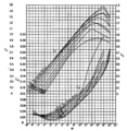  Fig 11.

• 

  Fig 12.

• 

  Figure 13.

• 

  Figure 14.

Attribution

This article incorporates text from a publication now in the public domain: Weick, Fred Ernest (1899). Aircraft propeller design. New York, McGraw-Hill Book Company, inc.. 

See also

• Circulation (fluid dynamics)
• Computational fluid dynamics

External links

• Blade Element Analysis for Propellers
• Helicopter Theory - Blade Element Theory in Forward Flight from Aerospaceweb.org
• Blade element theory
• Stefan Drzewiecki 1903
• QBlade: Open Source Blade Element Method Software from H.F.I. TU Berlin
• NASA-TM-102219: A survey of nonuniform inflow models for rotorcraft flight dynamics and control applications, by Robert Chen, NASA

References

- ↑ 1.0 1.1 Froude, William (11 April 1878). "The Elementary Relation between Pitch, Slip, and Propulsive Efficiency". Inst. Naval Architects 19: 47. https://babel.hathitrust.org/cgi/pt?id=iau.31858019833668&seq=81.
- ↑ This fact, which is not generally known in English-speaking countries, was called to the author’s attention by Prof. F. W. Pawlowski of the University of Michigan. Drzewiecki’s first French paper on his theory was published in 1892. He wrote in all seven papers on aircraft propulsion which were presented to l’Academie des Sciences, l’Association Technique Maritime, and Le Congrès International d’Architecture et de Construction Navale, held on July 15, 1900. He finally wrote a book summing up all of his work called "Théorie Générale de l’Hé1ice Propulsive," published in 1920 by Gauthier-Villars in Paris.
- ↑ Drzewiecki suggested that the airfoil characteristics could be obtained from tests on special model propellers.
- ↑ Glauert, H (1926). Aerofoil and Airscrew Theory. Cambridge University Press.
- ↑ C. N. H., Lock; Bateman, H.; Townend, H. C. H. (1924). Experiments to Verify the Independence of the Elements of an Airscrew Blade. British R. and M. 953.
- ↑ 6.0 6.1 Fage, A.; Howard, R. G. (1921). A Consideration of Airscrew Theory in the Light of Data Derived from an Experimental Investigation of the Distribution of Pressure over the Entire Surface of an Airscrew Blade, and also over Airfoils of Appropriate Shapes. British R. and M. 681.
- ↑ An Analysis of the Family of Airscrews by Means of the Vortex Theory and Measurements of Total Head, by C. N. H. Lock, and H. Bateman, British R. and M. 892, 1923.
- ↑ Comparison of Model Propeller Tests with Airfoil Theory, by William F. Durand, and E. P. Lesley, N.A.C.A .T.R. 196, 1924.
- ↑ Durand, W. F. (1926). Tests on Thirteen Navy Type Model Propellers. N.A.C.A .T.R. 237. propeller model C.