Physics:Burgers vortex
In fluid dynamics, the Burgers vortex or Burgers–Rott vortex is an exact solution to the Navier–Stokes equations governing viscous flow, named after Jan Burgers[1] and Nicholas Rott.[2] The Burgers vortex describes a stationary, self-similar flow. An inward, radial flow, tends to concentrate vorticity in a narrow column around the symmetry axis, while an axial stretching causes the vorticity to increase. At the same time, viscous diffusion tends to spread the vorticity. The stationary Burgers vortex arises when the three effects are in balance.
The Burgers vortex, apart from serving as an illustration of the vortex stretching mechanism, may describe such flows as tornados, where the vorticity is provided by continuous convection-driven vortex stretching.
Flow field
The flow for the Burgers vortex is described in cylindrical coordinates. Assuming axial symmetry (no -dependence), the flow field associated with the axisymmetric stagnation point flow is considered:
where (strain rate) and (circulation) are constants. The flow satisfies the continuity equation by the two first of the above equations. The azimuthal momentum equation of the Navier–Stokes equations then reduces to[3]
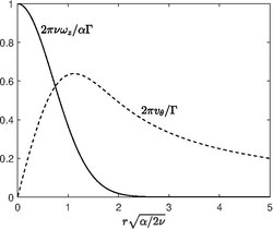
where is the kinematic viscosity of the fluid. The equation is integrated with the condition so that at infinity the solution behaves like a potential vortex, but at finite location, the flow is rotational. The choice ensures at the axis. The solution is
The vorticity equation only gives a non-trivial component in the -direction, given by
Intuitively the flow can be understood by looking at the three terms in the vorticity equation for ,
The first term on the right-hand side of the above equation corresponds to vortex stretching which intensifies the vorticity of the vortex core due to the axial-velocity component . The intensified vorticity tries to diffuse outwards radially due to the second term on the right-hand side, but is prevented by radial vorticity convection due to that emerges on the left-hand side of the above equation. The three-way balance establishes a steady solution. The Burgers vortex is a stable solution of the Navier–Stokes equations.[4]
One of the important property of the Burgers vortex that was shown by Jan Burgers is that the total viscous dissipation rate per unit axial length is independent of the viscosity, indicating that dissipation by the Burgers vortex is non-zero even in the limit . For this reason, it serves as a suitable candidate in modelling and understanding stretched-vortex tubes observed in turbulent flows. The total dissipation rate per unit axial length is, in incompressible flows, simply equal to the total enstrophy per unit length, which is given by[5]
Unsteady evolution to Burgers's vortex
An exact solution of the time dependent Navier Stokes equations for arbitrary function is available. In particular, when is constant, the vorticity field with an arbitrary initial distribution is given by[6]
As , the asymptotic behaviour is given by
Thus, provided , an arbitrary vorticity distribution approaches the Burgers' vortex.[7] If , say in the case where the initial condition is composed of two equal and opposite vortices, then the first term is zero and the second term implies that vorticity decays to zero as
Burgers vortex layer

Burgers vortex layer or Burgers vortex sheet is a strained shear layer, which is a two-dimensional analogue of Burgers vortex. This is also an exact solution of the Navier–Stokes equations, first described by Albert A. Townsend in 1951.[8] The velocity field expressed in the Cartesian coordinates are
where is the strain rate, and . The value is interpreted as the vortex sheet strength. The vorticity equation only gives a non-trivial component in the -direction, given by
The Burgers vortex sheet is shown to be unstable to small disturbances by K. N. Beronov and S. Kida[9] thereby undergoing Kelvin–Helmholtz instability initially, followed by second instabilities[10][11] and possibly transitioning to Kerr–Dold vortices at moderately large Reynolds numbers, but becoming turbulent at large Reynolds numbers.
Non-axisymmetric Burgers vortices
Non-axisymmetric Burgers' vortices emerge in non-axisymmetric strained flows. The theory for non-axisymmetric Burgers's vortex for small vortex Reynolds numbers was developed by A. C. Robinson and Philip Saffman in 1984,[4] whereas Keith Moffatt, S. Kida and K. Ohkitani has developed the theory for in 1994.[12] The structure of non-axisymmetric Burgers' vortices for arbitrary values of vortex Reynolds number can be discussed through numerical integrations.[13] The velocity field takes the form
subjected to the condition . Without loss of generality, one assumes and . The vortex cross-section lies in plane, providing a non-zero vorticity component in the direction
The axisymmetric Burgers' vortex is recovered when whereas the Burgers' vortex layer is recovered when and .
Burgers vortex in cylindrical stagnation surfaces
Explicit solution of the Navier–Stokes equations for the Burgers vortex in stretched cylindrical stagnation surfaces was solved by P. Rajamanickam and A. D. Weiss.[14] The solution is expressed in the cylindrical coordinate system as follows
where is the strain rate, is the radial location of the cylindrical stagnation surface, is the circulation and is the regularized gamma function. This solution is nothing but the Burgers' vortex in the presence of a line source with source strength . The vorticity equation only gives a non-trivial component in the -direction, given by
where in the above expression is the gamma function. As , the solution reduces to Burgers' vortex solution and as , the solution becomes the Burgers' vortex layer solution. Explicit solution for Sullivan vortex in cylindrical stagnation surface also exists.
See also
- Sullivan vortex
- Kerr–Dold vortex
References
- ↑ Burgers, J. M. (1948). A mathematical model illustrating the theory of turbulence. In Advances in applied mechanics (Vol. 1, pp. 171–199). Elsevier.
- ↑ Rott, N. (1958). On the viscous core of a line vortex. Zeitschrift für angewandte Mathematik und Physik ZAMP, 9(5–6), 543–553.
- ↑ Drazin, P. G., & Riley, N. (2006). The Navier–Stokes equations: a classification of flows and exact solutions (No. 334). Cambridge University Press.
- ↑ 4.0 4.1 Robinson, A. C., & Saffman, P. G. (1984). Stability and structure of stretched vortices. Studies in applied mathematics, 70(2), 163–181.
- ↑ Moffatt, H. K. (2011). A brief introduction to vortex dynamics and turbulence. In Environmental hazards: the fluid dynamics and geophysics of extreme events (pp. 1-27).
- ↑ Kambe, T. (1984). Axisymmetric vortex solution of Navier–Stokes equation. Journal of the Physical Society of Japan, 53(1), 13–15.
- ↑ Batchelor, G. K. (1967). An introduction to fluid dynamics. Cambridge university press. Page 272.
- ↑ Townsend, A. A. (1951). On the fine-scale structure of turbulence. Proceedings of the Royal Society of London. Series A. Mathematical and Physical Sciences, 208(1095), 534–542.
- ↑ Beronov, K. N., & Kida, S. (1996). Linear two-dimensional stability of a Burgers vortex layer. Physics of Fluids, 8(4), 1024–1035.
- ↑ Neu, J. C. (1984). The dynamics of stretched vortices. Journal of Fluid Mechanics, 143, 253–276.
- ↑ Lin, S. C., & Corcos, G. M. (1984). The mixing layer: deterministic models of a turbulent flow. Part 3. The effect of plane strain on the dynamics of streamwise vortices. Journal of Fluid Mechanics, 141, 139–178.
- ↑ Moffatt, H. K., Kida, S., & Ohkitani, K. (1994). Stretched vortices–the sinews of turbulence; large-Reynolds-number asymptotics. Journal of Fluid Mechanics, 259, 241–264.
- ↑ Prochazka, A., & Pullin, D. I. (1998). Structure and stability of non-symmetric Burgers vortices. Journal of Fluid Mechanics, 363, 199–228.
- ↑ Rajamanickam, P., & Weiss, A. D. (2021). Steady axisymmetric vortices in radial stagnation flows. The Quarterly Journal of Mechanics and Applied Mathematics, 74(3), 367–378.
 |  |
