Exponential integral
_with_n%3D2_in_the_complex_plane_from_-2-2i_to_2%2B2i_with_colors_created_with_Mathematica_13.1_function_ComplexPlot3D.svg)
In mathematics, the exponential integral Ei is a special function on the complex plane.
It is defined as one particular definite integral of the ratio between an exponential function and its argument.
Definitions
For real non-zero values of x, the exponential integral Ei(x) is defined as
The Risch algorithm shows that Ei is not an elementary function. The definition above can be used for positive values of x, but the integral has to be understood in terms of the Cauchy principal value due to the singularity of the integrand at zero.
For complex values of the argument, the definition becomes ambiguous due to branch points at 0 and .[1] Instead of Ei, the following notation is used,[2]
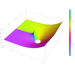
Plot of the exponential integral function Ei(z) in the complex plane from -2-2i to 2+2i with colors created with Mathematica 13.1 function ComplexPlot3D
_in_the_complex_plane_from_-2-2i_to_2%2B2i_with_colors_created_with_Mathematica_13.1_function_ComplexPlot3D.svg)
For positive values of x, we have .
In general, a branch cut is taken on the negative real axis and E1 can be defined by analytic continuation elsewhere on the complex plane.
For positive values of the real part of , this can be written[3]
The behaviour of E1 near the branch cut can be seen by the following relation:[4]
Properties
Several properties of the exponential integral below, in certain cases, allow one to avoid its explicit evaluation through the definition above.
Convergent series

For real or complex arguments off the negative real axis, can be expressed as[5]
where is the Euler–Mascheroni constant. The sum converges for all complex , and we take the usual value of the complex logarithm having a branch cut along the negative real axis.
This formula can be used to compute with floating point operations for real between 0 and 2.5. For , the result is inaccurate due to cancellation.
A faster converging series was found by Ramanujan:[6]
Asymptotic (divergent) series

Unfortunately, the convergence of the series above is slow for arguments of larger modulus. For example, more than 40 terms are required to get an answer correct to three significant figures for .[7] However, for positive values of x, there is a divergent series approximation that can be obtained by integrating by parts:[8]
The relative error of the approximation above is plotted on the figure to the right for various values of , the number of terms in the truncated sum ( in red, in pink).
Asymptotics beyond all orders

Using integration by parts, we can obtain an explicit formula[9] For any fixed , the absolute value of the error term decreases, then increases. The minimum occurs at , at which point . This bound is said to be "asymptotics beyond all orders".
Exponential and logarithmic behavior: bracketing

From the two series suggested in previous subsections, it follows that behaves like a negative exponential for large values of the argument and like a logarithm for small values. For positive real values of the argument, can be bracketed by elementary functions as follows:[10]
The left-hand side of this inequality is shown in the graph to the left in blue; the central part is shown in black and the right-hand side is shown in red.
Definition by Ein
Both and can be written more simply using the entire function [11] defined as
(note that this is just the alternating series in the above definition of ). Then we have
The function is related to the exponential generating function of the harmonic numbers:
Relation with other functions
Kummer's equation
is usually solved by the confluent hypergeometric functions and But when and that is,
we have
for all z. A second solution is then given by E1(−z). In fact,
with the derivative evaluated at Another connexion with the confluent hypergeometric functions is that E1 is an exponential times the function U(1,1,z):
The exponential integral is closely related to the logarithmic integral function li(x) by the formula
for non-zero real values of .
The series expansion of the exponential integral immediately gives rise to an expression in terms of the generalized hypergeometric function :
Generalization
The exponential integral may also be generalized to
which can be written as a special case of the upper incomplete gamma function:[12]
The generalized form is sometimes called the Misra function[13] , defined as
Many properties of this generalized form can be found in the NIST Digital Library of Mathematical Functions.
Including a logarithm defines the generalized integro-exponential function[14]
Derivatives
The derivatives of the generalised functions can be calculated by means of the formula [15]
Note that the function is easy to evaluate (making this recursion useful), since it is just .[16]
Exponential integral of imaginary argument

If is imaginary, it has a nonnegative real part, so we can use the formula
to get a relation with the trigonometric integrals and :
The real and imaginary parts of are plotted in the figure to the right with black and red curves.
Approximations
There have been a number of approximations for the exponential integral function. These include:
- The Swamee and Ohija approximation[17] where
- The Allen and Hastings approximation [17][18] where
- The continued fraction expansion [18]
- The approximation of Barry et al. [19] where: with being the Euler–Mascheroni constant.
Inverse function of the Exponential Integral
We can express the Inverse function of the exponential integral in power series form:[20]
where is the Ramanujan–Soldner constant and is polynomial sequence defined by the following recurrence relation:
For , and we have the formula :
Applications
- Time-dependent heat transfer
- Nonequilibrium groundwater flow in the Theis solution (called a well function)
- Radiative transfer in stellar and planetary atmospheres
- Radial diffusivity equation for transient or unsteady state flow with line sources and sinks
- Solutions to the neutron transport equation in simplified 1-D geometries[21]
- Solutions to the Trachenko-Zaccone nonlinear differential equation for the stretched exponential function in the relaxation of amorphous solids and glass transition[22][23]
See also
Notes
- ↑ Abramowitz and Stegun, p. 228
- ↑ Abramowitz and Stegun, p. 228, 5.1.1
- ↑ Abramowitz and Stegun, p. 228, 5.1.4 with n = 1
- ↑ Abramowitz and Stegun, p. 228, 5.1.7
- ↑ Abramowitz and Stegun, p. 229, 5.1.11
- ↑ Andrews and Berndt, p. 130, 24.16
- ↑ Bleistein and Handelsman, p. 2
- ↑ Bleistein and Handelsman, p. 3
- ↑ O’Malley, Robert E. (2014), O'Malley, Robert E., ed., "Asymptotic Approximations" (in en), Historical Developments in Singular Perturbations (Cham: Springer International Publishing): pp. 27–51, doi:10.1007/978-3-319-11924-3_2, ISBN 978-3-319-11924-3, https://doi.org/10.1007/978-3-319-11924-3_2, retrieved 2023-05-04
- ↑ Abramowitz and Stegun, p. 229, 5.1.20
- ↑ Abramowitz and Stegun, p. 228, see footnote 3.
- ↑ Abramowitz and Stegun, p. 230, 5.1.45
- ↑ After Misra (1940), p. 178
- ↑ Milgram (1985)
- ↑ Abramowitz and Stegun, p. 230, 5.1.26
- ↑ Abramowitz and Stegun, p. 229, 5.1.24
- ↑ 17.0 17.1 Giao, Pham Huy (2003-05-01). "Revisit of Well Function Approximation and An Easy Graphical Curve Matching Technique for Theis' Solution". Ground Water 41 (3): 387–390. doi:10.1111/j.1745-6584.2003.tb02608.x. ISSN 1745-6584. PMID 12772832. Bibcode: 2003GrWat..41..387G.
- ↑ 18.0 18.1 Tseng, Peng-Hsiang; Lee, Tien-Chang (1998-02-26). "Numerical evaluation of exponential integral: Theis well function approximation". Journal of Hydrology 205 (1–2): 38–51. doi:10.1016/S0022-1694(97)00134-0. Bibcode: 1998JHyd..205...38T.
- ↑ Barry, D. A; Parlange, J. -Y; Li, L (2000-01-31). "Approximation for the exponential integral (Theis well function)". Journal of Hydrology 227 (1–4): 287–291. doi:10.1016/S0022-1694(99)00184-5. Bibcode: 2000JHyd..227..287B.
- ↑ "Inverse function of the Exponential Integral Ei-1(x)". https://math.stackexchange.com/questions/4901881/inverse-function-of-the-exponential-integral-mathrmei-1x.
- ↑ George I. Bell; Samuel Glasstone (1970). Nuclear Reactor Theory. Van Nostrand Reinhold Company.
- ↑ Trachenko, K.; Zaccone, A. (2021-06-14). "Slow stretched-exponential and fast compressed-exponential relaxation from local event dynamics" (in en). Journal of Physics: Condensed Matter 33: 315101. doi:10.1088/1361-648X/ac04cd. ISSN 0953-8984. https://iopscience.iop.org/article/10.1088/1361-648X/ac04cd.
- ↑ Ginzburg, V. V.; Gendelman, O. V.; Zaccone, A. (2024-02-23). "Unifying Physical Framework for Stretched-Exponential, Compressed-Exponential, and Logarithmic Relaxation Phenomena in Glassy Polymers" (in en). Macromolecules 57 (5): 2520–2529. doi:10.1021/acs.macromol.3c02480. ISSN 0024-9297. https://pubs.acs.org/doi/full/10.1021/acs.macromol.3c02480.
References
- Abramowitz, Milton; Irene Stegun (1964). Handbook of Mathematical Functions with Formulas, Graphs, and Mathematical Tables. Abramowitz and Stegun. New York: Dover. ISBN 978-0-486-61272-0. https://archive.org/details/handbookofmathe000abra., Chapter 5.
- Bender, Carl M.; Steven A. Orszag (1978). Advanced mathematical methods for scientists and engineers. McGraw–Hill. ISBN 978-0-07-004452-4.
- Bleistein, Norman; Richard A. Handelsman (1986). Asymptotic Expansions of Integrals. Dover. ISBN 978-0-486-65082-1.
- Andrews, George E.; Berndt, Bruce C. (2013), Ramanujan's lost notebook. Part IV, Berlin, New York: Springer-Verlag, ISBN 978-1-4614-4080-2
- Busbridge, Ida W. (1950). "On the integro-exponential function and the evaluation of some integrals involving it". Quart. J. Math. (Oxford) 1 (1): 176–184. doi:10.1093/qmath/1.1.176. Bibcode: 1950QJMat...1..176B.
- Stankiewicz, A. (1968). "Tables of the integro-exponential functions". Acta Astronomica 18: 289. Bibcode: 1968AcA....18..289S.
- Sharma, R. R.; Zohuri, Bahman (1977). "A general method for an accurate evaluation of exponential integrals E1(x), x>0". J. Comput. Phys. 25 (2): 199–204. doi:10.1016/0021-9991(77)90022-5. Bibcode: 1977JCoPh..25..199S.
- Kölbig, K. S. (1983). "On the integral exp(−μt)tν−1logmt dt". Math. Comput. 41 (163): 171–182. doi:10.1090/S0025-5718-1983-0701632-1.
- Milgram, M. S. (1985). "The generalized integro-exponential function". Mathematics of Computation 44 (170): 443–458. doi:10.1090/S0025-5718-1985-0777276-4.
- Misra, Rama Dhar; Born, M. (1940). "On the Stability of Crystal Lattices. II". Mathematical Proceedings of the Cambridge Philosophical Society 36 (2): 173. doi:10.1017/S030500410001714X. Bibcode: 1940PCPS...36..173M.
- Chiccoli, C.; Lorenzutta, S.; Maino, G. (1988). "On the evaluation of generalized exponential integrals Eν(x)". J. Comput. Phys. 78 (2): 278–287. doi:10.1016/0021-9991(88)90050-2. Bibcode: 1988JCoPh..78..278C.
- Chiccoli, C.; Lorenzutta, S.; Maino, G. (1990). "Recent results for generalized exponential integrals". Computer Math. Applic. 19 (5): 21–29. doi:10.1016/0898-1221(90)90098-5. https://www.openaccessrepository.it/record/135675.
- MacLeod, Allan J. (2002). "The efficient computation of some generalised exponential integrals". J. Comput. Appl. Math. 148 (2): 363–374. doi:10.1016/S0377-0427(02)00556-3. Bibcode: 2002JCoAM.148..363M.
- Press, WH; Teukolsky, SA; Vetterling, WT; Flannery, BP (2007), "Section 6.3. Exponential Integrals", Numerical Recipes: The Art of Scientific Computing (3rd ed.), New York: Cambridge University Press, ISBN 978-0-521-88068-8, http://apps.nrbook.com/empanel/index.html#pg=266, retrieved 2011-08-09
- Temme, N. M. (2010), "Exponential, Logarithmic, Sine, and Cosine Integrals", in Olver, Frank W. J.; Lozier, Daniel M.; Boisvert, Ronald F. et al., NIST Handbook of Mathematical Functions, Cambridge University Press, ISBN 978-0-521-19225-5, http://dlmf.nist.gov/6
External links
- Hazewinkel, Michiel, ed. (2001), "Integral exponential function", Encyclopedia of Mathematics, Springer Science+Business Media B.V. / Kluwer Academic Publishers, ISBN 978-1-55608-010-4, https://www.encyclopediaofmath.org/index.php?title=p/i051440
- NIST documentation on the Generalized Exponential Integral
- Weisstein, Eric W.. "Exponential Integral". http://mathworld.wolfram.com/ExponentialIntegral.html.
- Weisstein, Eric W.. "En-Function". http://mathworld.wolfram.com/En-Function.html.
- Template:WolframFunctionsSite
- Exponential, Logarithmic, Sine, and Cosine Integrals in DLMF.
 |  |
