Physics:Cell lists
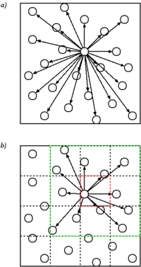
Cell lists (also sometimes referred to as cell linked-lists) is a data structure in molecular dynamics simulations to find all atom pairs within a given cut-off distance of each other. These pairs are needed to compute the short-range non-bonded interactions in a system, such as Van der Waals forces or the short-range part of the electrostatic interaction when using Ewald summation.
Algorithm

Cell lists work by subdividing the simulation domain into cells with an edge length greater than or equal to the cut-off radius of the interaction to be computed. The particles are sorted into these cells and the interactions are computed between particles in the same or neighbouring cells.
In its most basic form, the non-bonded interactions for a cut-off distance are computed as follows:
- for all neighbouring cell pairs do
- for all do
- for all do
- if then
- Compute the interaction between and .
- end if
- if then
- end for
- for all do
- end for
- for all do
- end for
Since the cell length is at least in all dimensions, no particles within of each other can be missed.
Given a simulation with particles with a homogeneous particle density, the number of cells is proportional to and inversely proportional to the cut-off radius (i.e. if increases, so does the number of cells). The average number of particles per cell therefore does not depend on the total number of particles. The cost of interacting two cells is in . The number of cell pairs is proportional to the number of cells which is again proportional to the number of particles . The total cost of finding all pairwise distances within a given cut-off is in , which is significantly better than computing the pairwise distances naively.
Periodic boundary conditions
In most simulations, periodic boundary conditions are used to avoid imposing artificial boundary conditions. Using cell lists, these boundaries can be implemented in two ways.
Ghost cells

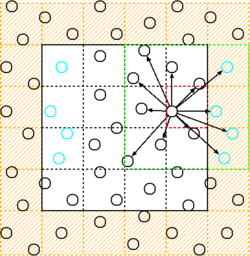
In the ghost cells approach, the simulation box is wrapped in an additional layer of cells. These cells contain periodically wrapped copies of the corresponding simulation cells inside the domain.
Although the data—and usually also the computational cost—is doubled for interactions over the periodic boundary, this approach has the advantage of being straightforward to implement and very easy to parallelize, since cells will only interact with their geographical neighbours.
Periodic wrapping
Instead of creating ghost cells, cell pairs that interact over a periodic boundary can also use a periodic correction vector . This vector, which can be stored or computed for every cell pair , contains the correction which needs to be applied to "wrap" one cell around the domain to neighbour the other. The pairwise distance between two particles and is then computed as
- .
This approach, although more efficient than using ghost cells, is less straightforward to implement (the cell pairs need to be identified over the periodic boundaries and the vector needs to be computed/stored).
Improvements
Despite reducing the computational cost of finding all pairs within a given cut-off distance from to , the cell list algorithm listed above still has some inefficiencies.
Consider a computational cell in three dimensions with edge length equal to the cut-off radius . The pairwise distance between all particles in the cell and in one of the neighbouring cells is computed. The cell has 26 neighbours: 6 sharing a common face, 12 sharing a common edge and 8 sharing a common corner. Of all the pairwise distances computed, only about 16% will actually be less than or equal to . In other words, 84% of all pairwise distance computations are spurious.
One way of overcoming this inefficiency is to partition the domain into cells of edge length smaller than . The pairwise interactions are then not just computed between neighboring cells, but between all cells within of each other (first suggested in [1] and implemented and analysed in [2][3] and [4]). This approach can be taken to the limit wherein each cell holds at most one single particle, therefore reducing the number of spurious pairwise distance evaluations to zero. This gain in efficiency, however, is quickly offset by the number of cells that need to be inspected for every interaction with a cell , which, for example in three dimensions, grows cubically with the inverse of the cell edge length. Setting the edge length to , however, already reduces the number of spurious distance evaluations to 63%.
Another approach is outlined and tested in Gonnet,[5] in which the particles are first sorted along the axis connecting the cell centers. This approach generates only about 40% spurious pairwise distance computations, yet carries an additional cost due to sorting the particles.
See also
References
- ↑ Allen, M. P.; D. J. Tildesley (1987). Computer Simulation of Liquids. Oxford: Clarendon Press.
- ↑ Mattson, W.; B. M. Rice (1999). "Near-neighbor calculations using a modified cell-linked list method". Computer Physics Communications 119 (2–3): 135. doi:10.1016/S0010-4655(98)00203-3. Bibcode: 1999CoPhC.119..135M.
- ↑ Yao, Z.; Wang, J.-S.; Liu, G.-R.; Cheng, M (2004). "Improved neighbor list algorithm in molecular simulations using cell decomposition and data sorting method". Computer Physics Communications 161 (1–2): 27–35. doi:10.1016/j.cpc.2004.04.004. Bibcode: 2004CoPhC.161...27Y.
- ↑ Heinz, T. N.; Hünenberger, P. H. (2004). "A fast pairlist-construction algorithm for molecular simulations under periodic boundary conditions". Journal of Computational Chemistry 25 (12): 1474–86. doi:10.1002/jcc.20071. PMID 15224391.
- ↑ Gonnet, Pedro (2007). "A Simple Algorithm to Accelerate the Computation of Non-Bonded Interactions in Cell-Based Molecular Dynamics Simulations". Journal of Computational Chemistry 28 (2): 570–573. doi:10.1002/jcc.20563. PMID 17183605.
 |
