Physics:Standard linear solid model
The standard linear solid (SLS), also known as the Zener model after Clarence Zener,[1] is a method of modeling the behavior of a viscoelastic material using a linear combination of springs and dashpots to represent elastic and viscous components, respectively. Often, the simpler Maxwell model and the Kelvin–Voigt model are used. These models often prove insufficient, however; the Maxwell model does not describe creep or recovery, and the Kelvin–Voigt model does not describe stress relaxation. SLS is the simplest model that predicts both phenomena.
Definition
Materials undergoing strain are often modeled with mechanical components, such as springs (restorative force component) and dashpots (damping component).
Connecting a spring and damper in series yields a model of a Maxwell material while connecting a spring and damper in parallel yields a model of a Kelvin–Voigt material.[2] In contrast to the Maxwell and Kelvin–Voigt models, the SLS is slightly more complex, involving elements both in series and in parallel. Springs, which represent the elastic component of a viscoelastic material, obey Hooke's law:
where σ is the applied stress, E is the Young's modulus of the material, and ε is the strain. The spring represents the elastic component of the model's response.[2]
Dashpots represent the viscous component of a viscoelastic material. In these elements, the applied stress varies with the time rate of change of the strain:
where η is viscosity of the dashpot component.
Solving the model
In order to model this system, the following physical relations must be realized:
For parallel components: , and .[2]
For series components: , and .[2]
Maxwell representation

This model consists of two systems in parallel. The first, referred to as the Maxwell arm, contains a spring () and dashpot (viscosity ) in series.[2] The other system contains only a spring ().
These relationships help relate the various stresses and strains in the overall system and the Maxwell arm:
where the subscripts , , and refer to Maxwell, dashpot, spring one and spring two, respectively.
Using these relationships, their time derivatives, and the above stress-strain relationships for the spring and dashpot elements, the system can be modeled as follows:
The equation can also be expressed as:
or, in dot notation:
The relaxation time, , is different for each material and is equal to
Kelvin-Voigt representation

This model consists of two systems in series. The first, referred to as the Kelvin arm, contains a spring () and dashpot (viscosity ) in parallel. The other system contains only a spring ().
These relationships help relate the various stresses and strains in the overall system and the Kelvin arm:
where the subscripts , , , and refer to Kelvin, dashpot, spring one, and spring two, respectively.
Using these relationships, their time derivatives, and the above stress-strain relationships for the spring and dashpot elements, the system can be modeled as follows:
or, in dot notation:
The retardation time, , is different for each material and is equal to
Model characteristics

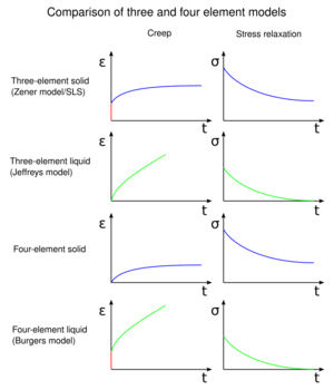
The standard linear solid model combines aspects of the Maxwell and Kelvin–Voigt models to accurately describe the overall behavior of a system under a given set of loading conditions. The behavior of a material applied to an instantaneous stress is shown as having an instantaneous component of the response. Instantaneous release of a stress also results in a discontinuous decrease in strain, as is expected. The shape of the time-dependent strain curve is true to the type of equation that characterizes the behavior of the model over time, depending upon how the model is loaded.
Although this model can be used to accurately predict the general shape of the strain curve, as well as behavior for long time and instantaneous loads, the model lacks the ability to accurately model material systems numerically.
The fluid model equivalent to the standard linear solid model includes a dashpot in series with the Kelvin–Voigt model and is called the Jeffreys model.[4]
See also
References
- ↑ Holm, Sverre (2024). Acoustic wave equations and four ways media may perturb the speed of sound. 1.3. University of Oslo. https://www.mn.uio.no/fysikk/english/people/aca/sverre/lecturenotes/waveequations-4speedsound.pdf.
- ↑ 2.0 2.1 2.2 2.3 2.4 David Roylance, "Engineering Viscoelasticity" (October 24, 2001) https://ocw.mit.edu/courses/materials-science-and-engineering/3-11-mechanics-of-materials-fall-1999/modules/MIT3_11F99_visco.pdf
- ↑ Krystyn J. Van Vliet, MIT course 3.032 Lecture, October 23, 2006 http://stellar.mit.edu/S/course/3/fa06/3.032/index.html
- ↑ Joseph, Daniel D. (2013-11-27) (in en). Fluid Dynamics of Viscoelastic Liquids. Springer Science & Business Media. ISBN 9781461244622. https://books.google.com/books?id=4IDkBwAAQBAJ&dq=jeffreys+element+viscoleastic&pg=PR5.
 |
