Polynomial kernel

Short description: Machine learning kernel function

Illustration of the mapping [math]\displaystyle{ \varphi }[/math]. On the left a set of samples in the input space, on the right the same samples in the feature space where the polynomial kernel [math]\displaystyle{ K(x,y) }[/math] (for some values of the parameters [math]\displaystyle{ c }[/math] and [math]\displaystyle{ d }[/math]) is the inner product. The hyperplane learned in feature space by an SVM is an ellipse in the input space.

In machine learning, the polynomial kernel is a kernel function commonly used with support vector machines (SVMs) and other kernelized models, that represents the similarity of vectors (training samples) in a feature space over polynomials of the original variables, allowing learning of non-linear models.

Intuitively, the polynomial kernel looks not only at the given features of input samples to determine their similarity, but also combinations of these. In the context of regression analysis, such combinations are known as interaction features. The (implicit) feature space of a polynomial kernel is equivalent to that of polynomial regression, but without the combinatorial blowup in the number of parameters to be learned. When the input features are binary-valued (booleans), then the features correspond to logical conjunctions of input features.

Definition

For degree-d polynomials, the polynomial kernel is defined as

[math]\displaystyle{ K(x,y) = (x^\mathsf{T} y + c)^{d} }[/math]

where x and y are vectors of size n in the input space, i.e. vectors of features computed from training or test samples and c ≥ 0 is a free parameter trading off the influence of higher-order versus lower-order terms in the polynomial. When c = 0, the kernel is called homogeneous. (A further generalized polykernel divides x^Ty by a user-specified scalar parameter a.)

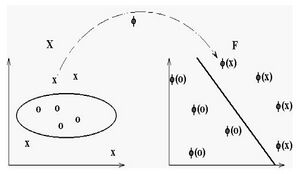
As a kernel, K corresponds to an inner product in a feature space based on some mapping φ:

[math]\displaystyle{ K(x,y) = \langle \varphi(x), \varphi(y) \rangle }[/math]

The nature of φ can be seen from an example. Let d = 2, so we get the special case of the quadratic kernel. After using the multinomial theorem (twice—the outermost application is the binomial theorem) and regrouping,

[math]\displaystyle{ K(x,y) = \left(\sum_{i=1}^n x_i y_i + c\right)^2 = \sum_{i=1}^n \left(x_i^2\right) \left(y_i^2 \right) + \sum_{i=2}^n \sum_{j=1}^{i-1} \left( \sqrt{2} x_i x_j \right) \left( \sqrt{2} y_i y_j \right) + \sum_{i=1}^n \left( \sqrt{2c} x_i \right) \left( \sqrt{2c} y_i \right) + c^2 }[/math]

From this it follows that the feature map is given by:

[math]\displaystyle{ \varphi(x) = \langle x_n^2, \ldots, x_1^2, \sqrt{2} x_n x_{n-1}, \ldots, \sqrt{2} x_n x_1, \sqrt{2} x_{n-1} x_{n-2}, \ldots, \sqrt{2} x_{n-1} x_{1}, \ldots, \sqrt{2} x_{2} x_{1}, \sqrt{2c} x_n, \ldots, \sqrt{2c} x_1, c \rangle }[/math]

generalizing for [math]\displaystyle{ \left(\mathbf{x}^{T}\mathbf{y} + c\right)^d }[/math], where [math]\displaystyle{ \mathbf{x}\in\mathbb{R}^{n} }[/math], [math]\displaystyle{ \mathbf{y}\in \mathbb{R}^{n} }[/math] and applying the multinomial theorem:

[math]\displaystyle{ \begin{alignat}{2} \left(\mathbf{x}^{T}\mathbf{y} + c\right)^d & = \sum_{j_1+j_2+\dots +j_{n+1}=d} \frac{\sqrt{d!}}{\sqrt{j_1! \cdots j_n! j_{n+1}!}} x_1^{j_1}\cdots x_n^{j_n} \sqrt{c}^{j_{n+1}} \frac{\sqrt{d!}}{\sqrt{j_1! \cdots j_n! j_{n+1}!}} y_1^{j_1}\cdots y_n^{j_n} \sqrt{c}^{j_{n+1}}\\ &=\varphi(\mathbf{x})^{T} \varphi(\mathbf{y}) \end{alignat} }[/math]

The last summation has [math]\displaystyle{ l_d=\tbinom {n+d}{d} }[/math] elements, so that:

[math]\displaystyle{ \varphi(\mathbf{x}) = \left(a_{1},\dots, a_{l},\dots,a_{l_d} \right ) }[/math]

where ,

[math]\displaystyle{ a_{l}=\frac{\sqrt{d!} }{\sqrt{j_1! \cdots j_n!j_{n+1}! }} x_1^{j_1}\cdots x_n^{j_n} \sqrt{c}^{j_{n+1}}\quad|\quad j_1+j_2+\dots+j_n +j_{n+1} = d }[/math]

Practical use

Although the RBF kernel is more popular in SVM classification than the polynomial kernel, the latter is quite popular in natural language processing (NLP). The most common degree is d = 2 (quadratic), since larger degrees tend to overfit on NLP problems.

Various ways of computing the polynomial kernel (both exact and approximate) have been devised as alternatives to the usual non-linear SVM training algorithms, including:

• full expansion of the kernel prior to training/testing with a linear SVM, i.e. full computation of the mapping φ as in polynomial regression;
• basket mining (using a variant of the apriori algorithm) for the most commonly occurring feature conjunctions in a training set to produce an approximate expansion;
• inverted indexing of support vectors.

One problem with the polynomial kernel is that it may suffer from numerical instability: when x^Ty + c < 1, K(x, y) = (x^Ty + c)^d tends to zero with increasing d, whereas when x^Ty + c > 1, K(x, y) tends to infinity.

References

- ↑ 1.0 1.1 1.2 Yoav Goldberg and Michael Elhadad (2008). splitSVM: Fast, Space-Efficient, non-Heuristic, Polynomial Kernel Computation for NLP Applications. Proc. ACL-08: HLT.
- ↑ "Archived copy". Archived from the original on 2013-04-15. https://web.archive.org/web/20130415231446/http://www.cs.tufts.edu/~roni/Teaching/CLT/LN/lecture18.pdf. Retrieved 2012-11-12.
- ↑ Shashua, Amnon (2009). "Introduction to Machine Learning: Class Notes 67577". arXiv:0904.3664v1 [cs.LG].
- ↑ 4.0 4.1 Lin, Chih-Jen (2012). "Machine learning software: design and practical use". Machine Learning Summer School. Kyoto. http://www.csie.ntu.edu.tw/~cjlin/talks/mlss_kyoto.pdf.
- ↑ 5.0 5.1 Chang, Yin-Wen; Hsieh, Cho-Jui; Chang, Kai-Wei; Ringgaard, Michael; Lin, Chih-Jen (2010). "Training and testing low-degree polynomial data mappings via linear SVM". Journal of Machine Learning Research 11: 1471–1490. http://jmlr.csail.mit.edu/papers/v11/chang10a.html.
- ↑ 6.0 6.1 Kudo, T.; Matsumoto, Y. (2003). "Fast methods for kernel-based text analysis". Proc. ACL.
- ↑ Lin, Chih-Jen (2012). "Shewchuk". Machine Learning Summer School. Kyoto. https://people.eecs.berkeley.edu/~jrs/189s21/lec/16.pdf.