Raised cosine distribution
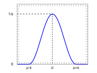
Probability density function | |||
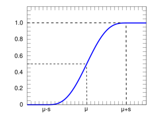
Cumulative distribution function | |||
Parameters |
[math]\displaystyle{ \mu\, }[/math](real) | ||
---|---|---|---|
Support | [math]\displaystyle{ x \in [\mu-s,\mu+s]\, }[/math] | ||
[math]\displaystyle{ \frac{1}{2s} \left[1+\cos\left(\frac{x-\mu}{s}\,\pi\right)\right]\,=\frac{1}{s}\operatorname{hvc}\left(\frac{x-\mu}{s}\,\pi\right)\, }[/math] | |||
CDF | [math]\displaystyle{ \frac{1}{2}\left[1+\frac{x-\mu}{s} +\frac{1}{\pi}\sin\left(\frac{x-\mu}{s}\,\pi\right)\right] }[/math] | ||
Mean | [math]\displaystyle{ \mu\, }[/math] | ||
Median | [math]\displaystyle{ \mu\, }[/math] | ||
Mode | [math]\displaystyle{ \mu\, }[/math] | ||
Variance | [math]\displaystyle{ s^2\left(\frac{1}{3}-\frac{2}{\pi^2}\right)\, }[/math] | ||
Skewness | [math]\displaystyle{ 0\, }[/math] | ||
Kurtosis | [math]\displaystyle{ \frac{6(90-\pi^4)}{5(\pi^2-6)^2}=-0.59376\ldots\, }[/math] | ||
MGF | [math]\displaystyle{ \frac{\pi^2\sinh(s t)}{st(\pi^2+s^2 t^2)}\,e^{\mu t} }[/math] | ||
CF | [math]\displaystyle{ \frac{\pi^2\sin(s t)}{st(\pi^2-s^2 t^2)}\,e^{i\mu t} }[/math] |
In probability theory and statistics, the raised cosine distribution is a continuous probability distribution supported on the interval [math]\displaystyle{ [\mu-s,\mu+s] }[/math]. The probability density function (PDF) is
- [math]\displaystyle{ f(x;\mu,s)=\frac{1}{2s} \left[1+\cos\left(\frac{x-\mu}{s}\,\pi\right)\right]\,=\frac{1}{s}\operatorname{hvc}\left(\frac{x-\mu}{s}\,\pi\right) \text{ for } \mu-s\le x\le\mu+s }[/math]
and zero otherwise. The cumulative distribution function (CDF) is
- [math]\displaystyle{ F(x;\mu,s)=\frac{1}{2}\left[1+\frac{x-\mu}{s} + \frac{1}{\pi} \sin\left(\frac{x-\mu}{s} \, \pi \right) \right] }[/math]
for [math]\displaystyle{ \mu-s \le x \le \mu+s }[/math] and zero for [math]\displaystyle{ x\lt \mu-s }[/math] and unity for [math]\displaystyle{ x\gt \mu+s }[/math].
The moments of the raised cosine distribution are somewhat complicated in the general case, but are considerably simplified for the standard raised cosine distribution. The standard raised cosine distribution is just the raised cosine distribution with [math]\displaystyle{ \mu=0 }[/math] and [math]\displaystyle{ s=1 }[/math]. Because the standard raised cosine distribution is an even function, the odd moments are zero. The even moments are given by:
- [math]\displaystyle{ \begin{align} \operatorname E(x^{2n}) & = \frac{1}{2}\int_{-1}^1 [1+\cos(x\pi)]x^{2n}\,dx = \int_{-1}^1 x^{2n} \operatorname{hvc}(x\pi)\,dx \\[5pt] & = \frac{1}{n+1}+\frac{1}{1+2n}\,_1F_2 \left(n+\frac{1}{2}; \frac{1}{2}, n+\frac{3}{2}; \frac{-\pi^2}{4} \right) \end{align} }[/math]
where [math]\displaystyle{ \,_1F_2 }[/math] is a generalized hypergeometric function.
See also
- Hann function
- Havercosine (hvc)
References
- Horst Rinne (2010). "Location-Scale Distributions – Linear Estimation and Probability Plotting Using MATLAB". p. 116. http://geb.uni-giessen.de/geb/volltexte/2010/7607/pdf/RinneHorst_LocationScale_2010.pdf.
Original source: https://en.wikipedia.org/wiki/Raised cosine distribution.
Read more |