Set estimation
In statistics, a random vector x is classically represented by a probability density function.
In a set-membership approach or set estimation, x is represented by a set X to which x is assumed to belong. This means that the support of the probability distribution function of x is included inside X. On the one hand, representing random vectors by sets makes it possible to provide fewer assumptions on the random variables (such as independence) and dealing with nonlinearities is easier. On the other hand, a probability distribution function provides a more accurate information than a set enclosing its support.
Set-membership estimation
Set membership estimation (or set estimation for short) is an estimation approach which considers that measurements are represented by a set Y (most of the time a box of where m is the number of measurements) of the measurement space. If p is the parameter vector and f is the model function, then the set of all feasible parameter vectors is
where P0 is the prior set for the parameters. Characterizing P corresponds to a set-inversion problem.[1]
Resolution
When f is linear the feasible set P can be described by linear inequalities and can be approximated using linear programming techniques.[2]
When f is nonlinear, the resolution can be performed using interval analysis. The feasible set P is then approximated by an inner and an outer subpavings. The main limitation of the method is its exponential complexity with respect to the number of parameters.[3]
Example
Consider the following model
where p1 and p2 are the two parameters to be estimated.

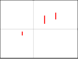
Assume that at times t1 = −1, t2 = 1, t3 = 2, the following interval measurements have been collected: as illustrated by Figure 1. The corresponding measurement set (here a box) is
The model function is defined by
The components of f are obtained using the model for each time measurement. After solving the set inversion problem, we get the approximation depicted on Figure 2. Red boxes are inside the feasible set P and blue boxes are outside P.

Recursive case
Set estimation can be used to estimate the state of a system described by state equations using a recursive implementation. When the system is linear, the corresponding feasible set for the state vector can be described by polytopes or by ellipsoids [4] .[5] When the system is nonlinear, the set can be enclosed by subpavings. [6]
Robust case
When outliers occur, the set estimation method generally returns an empty set. This is due to the fact that the intersection between sets of parameter vectors that are consistent with the ith data bar is empty. To be robust with respect to outliers, we generally characterize the set of parameter vectors that are consistent with all data bars except q of them. This is possible using the notion of q-relaxed intersection.
See also
References
- ↑ Jaulin, L.; Walter, E. (1993). "Guaranteed nonlinear parameter estimation via interval computations". Interval Computation. http://www.ensta-bretagne.fr/jaulin/paper_IntervalComp94.pdf.
- ↑ Walter, E.; Piet-Lahanier, H. (1989). "Exact Recursive Polyhedral Description of the Feasible Parameter Set for Bounded-Error Models". IEEE Transactions on Automatic Control 34 (8): 911–915. doi:10.1109/9.29443.
- ↑ Kreinovich, V.; Lakeyev, A.V.; Rohn, J.; Kahl, P.T. (1997). "Computational Complexity and Feasibility of Data Processing and Interval Computations". Reliable Computing 4 (4).
- ↑ Fogel, E.; Huang, Y.F. (1982). "On the Value of Information in System Identification - Bounded Noise Case". Automatica 18 (2): 229–238. doi:10.1016/0005-1098(82)90110-8.
- ↑ Schweppe, F.C. (1968). "Recursive State Estimation: unknown but Bounded Errors and System Inputs". IEEE Transactions on Automatic Control 13 (1): 22–28. doi:10.1109/tac.1968.1098790.
- ↑ Kieffer, M.; Jaulin, L.; Walter, E. (1998). "Guaranteed recursive nonlinear state estimation using interval Analysis". Proceedings of the 37th IEEE Conference on Decision and Control 4. http://www.ensta-bretagne.fr/jaulin/IEEEKalman.pdf.
 |
