Strip packing problem

The strip packing problem is a 2-dimensional geometric minimization problem. Given a set of axis-aligned rectangles and a strip of bounded width and infinite height, determine an overlapping-free packing of the rectangles into the strip minimizing its height. This problem is a cutting and packing problem and is classified as an Open Dimension Problem according to Wäscher et al.

This problem arises in the area of scheduling, where it models jobs, that require a contiguous portion of the memory over a given time period. Another example is the area of industrial manufacturing, where rectangular pieces need to be cut out of a sheet of material (e.g., cloth or paper) that has a fixed width but infinite length, and one wants to minimize the wasted material.

This problem was first studied in 1980. It is strongly-NP hard and there exists no polynomial time approximation algorithm with a ratio smaller than [math]\displaystyle{ 3/2 }[/math] unless [math]\displaystyle{ P = NP }[/math]. However, the best approximation ratio achieved so far (by a polynomial time algorithm by Harren et al.) is [math]\displaystyle{ (5/3 + \varepsilon) }[/math], imposing an open question whether there is an algorithm with approximation ratio [math]\displaystyle{ 3/2 }[/math].

Definition

An instance [math]\displaystyle{ I = (\mathcal{I},W) }[/math] of the strip packing problem consists of a strip with width [math]\displaystyle{ W = 1 }[/math] and infinite height, as well as a set [math]\displaystyle{ \mathcal{I} }[/math] of rectangular items. Each item [math]\displaystyle{ i \in \mathcal{I} }[/math] has a width [math]\displaystyle{ w_i \in (0,1] \cap \mathbb{Q} }[/math] and a height [math]\displaystyle{ h_i \in (0,1] \cap \mathbb{Q} }[/math]. A packing of the items is a mapping that maps each lower-left corner of an item [math]\displaystyle{ i \in \mathcal{I} }[/math] to a position [math]\displaystyle{ (x_i,y_i) \in ([0,1-w_i] \cap \mathbb{Q}) \times \mathbb{Q}_{\geq 0} }[/math] inside the strip. An inner point of a placed item [math]\displaystyle{ i \in \mathcal{I} }[/math] is a point from the set [math]\displaystyle{ \mathrm{inn}(i) = \{(x,y) \in \mathbb{Q} \times \mathbb{Q}| x_i \lt x \lt x_i + w_i, y_i \lt y \lt y_i + h_i\} }[/math]. Two (placed) items overlap if they share an inner point. The height of the packing is defined as [math]\displaystyle{ \max \{y_i+h_i | i \in \mathcal{I}\} }[/math]. The objective is to find an overlapping-free packing of the items inside the strip while minimizing the height of the packing.

This definition is used for all polynomial time algorithms. For pseudo-polynomial time and FPT-algorithms, the definition is slightly changed for the simplification of notation. In this case, all appearing sizes are integral. Especially the width of the strip is given by an arbitrary integer number larger than 1. Note that these two definitions are equivalent.

Variants

There are several variants of the strip packing problem that have been studied. These variants concern the geometry of the objects, dimension of the problem, if it is allowed to rotate the items, and the structure of the packing.

Geometry of the items: In the standard variant of this problem, the set of given items consists of rectangles. In an often considered subcase, all the items have to be squares. This variant was already considered in the first paper about strip packing. Additionally, variants have been studied where the shapes are circular or even irregular. In the latter case, we speak of irregular strip packing.

Dimension: When not mentioned differently the strip packing problem is a 2-dimensional problem. However, it also has been studied in three or even more dimensions. In this case, the objects are hyperrectangles, and the strip is open-ended in one dimension and bounded in the residual ones.

Rotation: In the classical strip packing problem, it is not allowed to rotate the items. However, variants have been studied where rotating by 90 degrees or even an arbitrary angle is allowed.

Structure of the packing: In the general strip packing problem, the structure of the packing is irrelevant. However, there are applications that have explicit requirements on the structure of the packing. One of these requirements is to be able to cut the items from the strip by horizontal or vertical edge to edge cuts. Packings that allow this kind of cutting are called guillotine packing.

Hardness

The strip packing problem contains the bin packing problem as a special case when all the items have the same height 1. For this reason, it is strongly NP-hard and there can be no polynomial time approximation algorithm, which has an approximation ratio smaller than [math]\displaystyle{ 3/2 }[/math] unless [math]\displaystyle{ P = NP }[/math]. Furthermore, unless [math]\displaystyle{ P = NP }[/math], there cannot be a pseudo-polynomial time algorithm that has an approximation ratio smaller than [math]\displaystyle{ 5/4 }[/math], which can be proven by a reduction from the strongly NP-complete 3-partition problem. Note that both lower bounds [math]\displaystyle{ 3/2 }[/math] and [math]\displaystyle{ 5/4 }[/math] also hold for the case that a rotation of the items by 90 degrees is allowed. Additionally, it was proven by Ashok et al. that strip packing is W[1]-hard when parameterized by the height of the optimal packing.

Properties of optimal solutions

There are two trivial lower bounds on optimal solutions. The first is the height of the largest item. Define [math]\displaystyle{ h_{\max}(I) := \max\{h(i) | i \in \mathcal{I}\} }[/math]. Then it holds that

[math]\displaystyle{ OPT(I) \geq h_{\max}(I) }[/math].

Another lower bound is given by the total area of the items. Define [math]\displaystyle{ \mathrm{AREA}(\mathcal{I}) := \sum_{i \in \mathcal{I}}h(i)w(i) }[/math] then it holds that

[math]\displaystyle{ OPT(I) \geq \mathrm{AREA}(\mathcal{I})/W }[/math].

The following two lower bounds take notice of the fact that certain items cannot be placed next to each other in the strip, and can be computed in [math]\displaystyle{ \mathcal{O}(n \log(n)) }[/math]. For the first lower bound assume that the items are sorted by non-increasing height. Define [math]\displaystyle{ k := \max \{i : \sum_{j = 1}^k w(j) \leq W\} }[/math]. For each [math]\displaystyle{ l \gt k }[/math] define [math]\displaystyle{ i(l) \leq k }[/math] the first index such that [math]\displaystyle{ w(l) + \sum_{j = 1}^{i(l)} w(j) \gt W }[/math]. Then it holds that

[math]\displaystyle{ OPT(I) \geq \max \{h(l) + h(i(l))| l \gt k \wedge w(l) + \sum_{j = 1}^{i(l)} w(j) \gt W\} }[/math].

For the second lower bound, partition the set of items into three sets. Let [math]\displaystyle{ \alpha \in [1, W/2]\cap \mathbb{N} }[/math] and define [math]\displaystyle{ \mathcal{I}_1(\alpha) := \{i \in \mathcal{I} | w(i) \gt W - \alpha\} }[/math], [math]\displaystyle{ \mathcal{I}_2(\alpha) := \{i \in \mathcal{I} | W - \alpha \geq w(i) \gt W/2\} }[/math], and [math]\displaystyle{ \mathcal{I}_3(\alpha) := \{i \in \mathcal{I} | W/2 \geq w(i) \gt \alpha \} }[/math]. Then it holds that

[math]\displaystyle{ OPT(I) \geq \max_{\alpha \in [1, W/2]\cap \mathbb{N}} \Bigg\{ \sum_{i \in \mathcal{I}_1(\alpha) \cup \mathcal{I}_2(\alpha)} h(i) + \left(\frac{\sum_{i \in \mathcal{I}_3(\alpha) h(i)w(i) - \sum_{i \in \mathcal{I}_2(\alpha)}(W -w(i))h(i)}}{W}\right)_+ \Bigg\} }[/math], where [math]\displaystyle{ (x)_+ := \max\{x,0\} }[/math] for each [math]\displaystyle{ x \in \mathbb{R} }[/math].

On the other hand, Steinberg has shown that the height of an optimal solution can be upper bounded by

[math]\displaystyle{ OPT(I) \leq 2\max\{h_{\max}(I),\mathrm{AREA}(\mathcal{I})/W\}. }[/math]

More precisely he showed that given a [math]\displaystyle{ W \geq w_{\max}(\mathcal{I}) }[/math] and a [math]\displaystyle{ H \geq h_{\max}(I) }[/math] then the items [math]\displaystyle{ \mathcal{I} }[/math] can be placed inside a box with width [math]\displaystyle{ W }[/math] and height [math]\displaystyle{ H }[/math] if

[math]\displaystyle{ WH \geq 2\mathrm{AREA}(\mathcal{I}) + (2w_{\max}(\mathcal{I}) - W)_+(2h_{\max}(I) - H)_+ }[/math], where [math]\displaystyle{ (x)_+ := \max\{x,0\} }[/math].

Polynomial time approximation algorithms

Since this problem is NP-hard, approximation algorithms have been studied for this problem. Most of the heuristic approaches have an approximation ratio between [math]\displaystyle{ 3 }[/math] and [math]\displaystyle{ 2 }[/math]. Finding an algorithm with a ratio below [math]\displaystyle{ 2 }[/math] seems hard, and the complexity of the corresponding algorithms increases regarding their running time and their descriptions. The smallest approximation ratio achieved so far is [math]\displaystyle{ (5/3+\varepsilon) }[/math].

Overview of polynomial time approximations

Year	Name	Approximation guarantee	Source
1980	Bottom-Up Left-Justified (BL)	[math]\displaystyle{ 3 OPT(I) }[/math]	Baker et al.
1980	Next-Fit Decreasing-Height (NFDH)	[math]\displaystyle{ 2 OPT(I) + h_{\max}(I) \leq 3 OPT(I) }[/math]	Coffman et al.
	First-Fit Decreasing-Height (FFDH)	[math]\displaystyle{ 1.7 OPT(I) + h_{\max}(I) \leq 2.7 OPT(I) }[/math]
	Split-Fit (SF)	[math]\displaystyle{ 1.5 OPT(I) + 2h_{\max}(I) }[/math]
1980		[math]\displaystyle{ 2 OPT(I) + h_{\max}(I)/2 \leq 2.5 OPT(I) }[/math]	Sleator
1981	Split Algorithm (SP)	[math]\displaystyle{ 3 OPT(I) }[/math]	Golan
	Mixed Algoritghm	[math]\displaystyle{ (4/3)OPT(I) + 7\frac{1}{18} h_{\max}(I) }[/math]
1981	Up-Down (UD)	[math]\displaystyle{ (5/4)OPT(I) + 6\frac{7}{8}h_{\max}(I) }[/math]	Baker et al.
1994	Reverse-Fit	[math]\displaystyle{ 2 OPT(I) }[/math]	Schiermeyer
1997		[math]\displaystyle{ 2 OPT(I) }[/math]	Steinberg
2000		[math]\displaystyle{ (1+\varepsilon) OPT(I) + \mathcal{O}(1/\varepsilon^2)h_{\max}(I) }[/math]	Kenyon, Rémila
2009		[math]\displaystyle{ 1.9396 OPT(I) }[/math]	Harren, van Stee
2009		[math]\displaystyle{ (1+\varepsilon) OPT(I) + h_{\max}(I) }[/math]	Jansen, Solis-Oba
2011		[math]\displaystyle{ (1+\varepsilon) OPT(I) + \mathcal{O}(\log(1/\varepsilon)/\varepsilon)h_{\max}(I) }[/math]	Bougeret et al.
2012		[math]\displaystyle{ (1+\varepsilon) OPT(I) + \mathcal{O}(\log(1/\varepsilon)/\varepsilon)h_{\max}(I) }[/math]	Sviridenko
2014		[math]\displaystyle{ (5/3+\varepsilon) OPT(I) }[/math]	Harren et al.

Bottom-up left-justified (BL)

An example of solutions generated by the Bottom-Up Left-Justified algorithm.

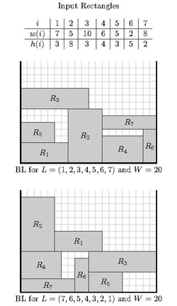
This algorithm was first described by Baker et al. It works as follows:

Let [math]\displaystyle{ L }[/math] be a sequence of rectangular items. The algorithm iterates the sequence in the given order. For each considered item [math]\displaystyle{ r \in L }[/math], it searches for the bottom-most position to place it and then shifts it as far to the left as possible. Hence, it places [math]\displaystyle{ r }[/math] at the bottom-most left-most possible coordinate [math]\displaystyle{ (x,y) }[/math] in the strip.

This algorithm has the following properties:

• The approximation ratio of this algorithm cannot be bounded by a constant. More precisely they showed that for each [math]\displaystyle{ M \gt 0 }[/math] there exists a list [math]\displaystyle{ L }[/math] of rectangular items ordered by increasing width such that [math]\displaystyle{ BL(L)/ OPT(L) \gt M }[/math], where [math]\displaystyle{ BL(L) }[/math] is the height of the packing created by the BL algorithm and [math]\displaystyle{ OPT(L) }[/math] is the height of the optimal solution for [math]\displaystyle{ L }[/math].
• If the items are ordered by decreasing widths, then [math]\displaystyle{ BL(L)/ OPT(L) \leq 3 }[/math].
• If the item are all squares and are ordered by decreasing widths, then [math]\displaystyle{ BL(L)/ OPT(L) \leq 2 }[/math].
• For any [math]\displaystyle{ \delta \gt 0 }[/math], there exists a list [math]\displaystyle{ L }[/math] of rectangles ordered by decreasing widths such that [math]\displaystyle{ BL(L)/ OPT(L) \gt 3 - \delta }[/math].
• For any [math]\displaystyle{ \delta \gt 0 }[/math], there exists a list [math]\displaystyle{ L }[/math] of squares ordered by decreasing widths such that [math]\displaystyle{ BL(L)/ OPT(L) \gt 2 - \delta }[/math].
• For each [math]\displaystyle{ \varepsilon \in (0,1] }[/math], there exists an instance containing only squares where each order of the squares [math]\displaystyle{ L }[/math] has a ratio of [math]\displaystyle{ BL(L)/ OPT(L) \gt \frac{12}{11 +\varepsilon} }[/math], i.e., there exist instances where BL does not find the optimum even when iterating all possible orders of the items.

Next-fit decreasing-height (NFDH)

An example for NFDH and FFDH applied to the same instance

This algorithm was first described by Coffman et al. in 1980 and works as follows:

Let [math]\displaystyle{ \mathcal{I} }[/math] be the given set of rectangular items. First, the algorithm sorts the items by order of nonincreasing height. Then, starting at position [math]\displaystyle{ (0,0) }[/math], the algorithm places the items next to each other in the strip until the next item will overlap the right border of the strip. At this point, the algorithm defines a new level at the top of the tallest item in the current level and places the items next to each other in this new level.

This algorithm has the following properties:

• The running time can be bounded by [math]\displaystyle{ \mathcal{O}(|\mathcal{I}| \log(|\mathcal{I}|)) }[/math] and if the items are already sorted even by [math]\displaystyle{ \mathcal{O}(|\mathcal{I}|) }[/math].
• For every set of items [math]\displaystyle{ \mathcal{I} }[/math], it produces a packing of height [math]\displaystyle{ NFDH(\mathcal{I}) \leq 2 OPT(\mathcal{I}) + h_{\max} \leq 3 OPT(\mathcal{I}) }[/math], where [math]\displaystyle{ h_{\max} }[/math] is the largest height of an item in [math]\displaystyle{ \mathcal{I} }[/math].
• For every [math]\displaystyle{ \varepsilon \gt 0 }[/math] there exists a set of rectangles [math]\displaystyle{ \mathcal{I} }[/math] such that [math]\displaystyle{ NFDH(\mathcal{I}|) \gt (2-\varepsilon) OPT(\mathcal{I}). }[/math]
• The packing generated is a guillotine packing. This means the items can be obtained through a sequence of horizontal or vertical edge-to-edge cuts.

First-fit decreasing-height (FFDH)

This algorithm, first described by Coffman et al. in 1980, works similar to the NFDH algorithm. However, when placing the next item, the algorithm scans the levels from bottom to top and places the item in the first level on which it will fit. A new level is only opened if the item does not fit in any previous ones.

This algorithm has the following properties:

• The running time can be bounded by [math]\displaystyle{ \mathcal{O}(|\mathcal{I}|^2) }[/math], since there are at most [math]\displaystyle{ |\mathcal{I}| }[/math] levels.
• For every set of items [math]\displaystyle{ \mathcal{I} }[/math] it produces a packing of height [math]\displaystyle{ FFDH(\mathcal{I}) \leq 1.7 OPT(\mathcal{I}) + h_{\max} \leq 2.7 OPT(\mathcal{I}) }[/math], where [math]\displaystyle{ h_{\max} }[/math] is the largest height of an item in [math]\displaystyle{ \mathcal{I} }[/math].
• Let [math]\displaystyle{ m \geq 2 }[/math]. For any set of items [math]\displaystyle{ \mathcal{I} }[/math] and strip with width [math]\displaystyle{ W }[/math] such that [math]\displaystyle{ w(i) \leq W/m }[/math] for each [math]\displaystyle{ i \in \mathcal{I} }[/math], it holds that [math]\displaystyle{ FFDH(\mathcal{I}) \leq \left(1 + 1/m\right) OPT(\mathcal{I}) + h_{\max} }[/math]. Furthermore, for each [math]\displaystyle{ \varepsilon \gt 0 }[/math], there exists such a set of items [math]\displaystyle{ \mathcal{I} }[/math] with [math]\displaystyle{ FFDH(\mathcal{I}) \gt \left(1 + 1/m -\varepsilon\right)OPT(\mathcal{I}) }[/math].
• If all the items in [math]\displaystyle{ \mathcal{I} }[/math] are squares, it holds that [math]\displaystyle{ FFDH(\mathcal{I}) \leq (3/2) OPT(\mathcal{I}) + h_{\max} }[/math]. Furthermore, for each [math]\displaystyle{ \varepsilon \gt 0 }[/math], there exists a set of squares [math]\displaystyle{ \mathcal{I} }[/math] such that [math]\displaystyle{ FFDH(\mathcal{I}) \gt \left(3/2-\varepsilon\right)OPT(\mathcal{I}) }[/math].
• The packing generated is a guillotine packing. This means the items can be obtained through a sequence of horizontal or vertical edge-to-edge cuts.

The split-fit algorithm (SF)

This algorithm was first described by Coffman et al. For a given set of items [math]\displaystyle{ \mathcal{I} }[/math] and strip with width [math]\displaystyle{ W }[/math], it works as follows:

1. Determinate [math]\displaystyle{ m \in \mathbb{N} }[/math], the largest integer such that the given rectangles have width [math]\displaystyle{ W/m }[/math] or less.
2. Divide [math]\displaystyle{ \mathcal{I} }[/math] into two sets [math]\displaystyle{ \mathcal{I}_{wide} }[/math] and [math]\displaystyle{ \mathcal{I}_{narrow} }[/math], such that [math]\displaystyle{ \mathcal{I}_{wide} }[/math] contains all the items [math]\displaystyle{ i \in \mathcal{I} }[/math] with a width [math]\displaystyle{ w(i) \gt W/(m+1) }[/math] while [math]\displaystyle{ \mathcal{I}_{narrow} }[/math] contains all the items with [math]\displaystyle{ w(i) \leq W/(m+1) }[/math].
3. Order [math]\displaystyle{ \mathcal{I}_{wide} }[/math] and [math]\displaystyle{ \mathcal{I}_{narrow} }[/math] by nonincreasing height.
4. Pack the items in [math]\displaystyle{ \mathcal{I}_{wide} }[/math] with the FFDH algorithm.
5. Reorder the levels/shelves constructed by FFDH such that all the shelves with a total width larger than [math]\displaystyle{ W(m+1)/(m+2) }[/math] are below the more narrow ones.
6. This leaves a rectangular area [math]\displaystyle{ R }[/math] of with [math]\displaystyle{ W/(m+2) }[/math], next to more narrow levels/shelves, that contains no item.
7. Use the FFDH algorithm to pack the items in [math]\displaystyle{ \mathcal{I}_{narrow} }[/math] using the area [math]\displaystyle{ R }[/math] as well.

This algorithm has the following properties:

• For every set of items [math]\displaystyle{ \mathcal{I} }[/math] and the corresponding [math]\displaystyle{ m }[/math], it holds that [math]\displaystyle{ SF(\mathcal{I}) \leq (m+2)/(m+1)OPT(\mathcal{I}) + 2h_{\max} }[/math]. Note that for [math]\displaystyle{ m=1 }[/math], it holds that [math]\displaystyle{ SF(\mathcal{I}) \leq (3/2) OPT(\mathcal{I}) + 2h_{\max} }[/math]
• For each [math]\displaystyle{ \varepsilon \gt 0 }[/math], there is a set of items [math]\displaystyle{ \mathcal{I} }[/math] such that [math]\displaystyle{ SF(\mathcal{I}) \gt \left((m+2)/(m+1) -\varepsilon\right)OPT(\mathcal{I}) }[/math].

Sleator's algorithm

For a given set of items [math]\displaystyle{ \mathcal{I} }[/math] and strip with width [math]\displaystyle{ W }[/math], it works as follows:

1. Find all the items with a width larger than [math]\displaystyle{ W/2 }[/math] and stack them at the bottom of the strip (in random order). Call the total height of these items [math]\displaystyle{ h_0 }[/math]. All the other items will be placed above [math]\displaystyle{ h_0 }[/math].
2. Sort all the remaining items in nonincreasing order of height. The items will be placed in this order.
3. Consider the horizontal line at [math]\displaystyle{ h_0 }[/math] as a shelf. The algorithm places the items on this shelf in nonincreasing order of height until no item is left or the next one does not fit.
4. Draw a vertical line at [math]\displaystyle{ W/2 }[/math], which cuts the strip into two equal halves.
5. Let [math]\displaystyle{ h_l }[/math] be the highest point covered by any item in the left half and [math]\displaystyle{ h_r }[/math] the corresponding point on the right half. Draw two horizontal line segments of length [math]\displaystyle{ W/2 }[/math] at [math]\displaystyle{ h_l }[/math] and [math]\displaystyle{ h_r }[/math] across the left and the right half of the strip. These two lines build new shelves on which the algorithm will place the items, as in step 3. Choose the half which has the lower shelf and place the items on this shelf until no other item fits. Repeat this step until no item is left.

This algorithm has the following properties:

• The running time can be bounded by [math]\displaystyle{ \mathcal{O}(|\mathcal{I}| \log(|\mathcal{I}|)) }[/math] and if the items are already sorted even by [math]\displaystyle{ \mathcal{O}(|\mathcal{I}|) }[/math].
• For every set of items [math]\displaystyle{ \mathcal{I} }[/math] it produces a packing of height [math]\displaystyle{ A(\mathcal{I}) \leq 2 OPT(\mathcal{I}) + h_{\max}/2 \leq 2.5 OPT(\mathcal{I}) }[/math], where [math]\displaystyle{ h_{\max} }[/math] is the largest height of an item in [math]\displaystyle{ \mathcal{I} }[/math].

The split algorithm (SP)

This algorithm is an extension of Sleator's approach and was first described by Golan. It places the items in nonincreasing order of width. The intuitive idea is to split the strip into sub-strips while placing some items. Whenever possible, the algorithm places the current item [math]\displaystyle{ i }[/math] side-by-side of an already placed item [math]\displaystyle{ j }[/math]. In this case, it splits the corresponding sub-strip into two pieces: one containing the first item [math]\displaystyle{ j }[/math] and the other containing the current item [math]\displaystyle{ i }[/math]. If this is not possible, it places [math]\displaystyle{ i }[/math] on top of an already placed item and does not split the sub-strip.

This algorithm creates a set S of sub-strips. For each sub-strip s ∈ S we know its lower left corner s.xposition and s.yposition, its width s.width, the horizontal lines parallel to the upper and lower border of the item placed last inside this sub-strip s.upper and s.lower, as well as the width of it s.itemWidth.

function Split Algorithm (SP) is
    input: items  I, width of the strip W
    output: A packing of the items
    Sort I in nonincreasing order of widths;
    Define empty list S of sub-strips;
    Define a new sub-strip s with s.xposition = 0, s.yposition = 0, s.width = W, s.lower = 0, s.upper = 0, s.itemWidth = W;
    Add s to S;
    while I not empty do
        i := I.pop(); Removes widest item from I
        Define new list S_2 containing all the substrips with s.width - s.itemWidth ≥ i.width; 
        S_2 contains all sub-strips where i fits next to the already placed item
        if S_2 is empty then
            In this case, place the item on top of another one.
            Find the sub-strip s in S with smallest s.upper; i.e. the least filled sub-strip
            Place i at position (s.xposition, s.upper);
            Update s: s.lower := s.upper; s.upper := s.upper+i.height; s.itemWidth := i.width;
        else 
            In this case, place the item next to another one at the same level and split the corresponding sub-strip at this position.
            Find s ∈ S_2 with the smallest s.lower;
            Place i at position (s.xposition + s.itemWidth, s.lower);
            Remove s from S;
            Define two new sub-strips s1 and s2 with 
            s1.xposition = s.xposition, s1.yposition = s.upper, s1.width = s.itemWidth, s1.lower = s.upper, s1.upper = s.upper, s1.itemWidth = s.itemWidth;
            s2.xposition = s.xposition+s.itemWidth, s2.yposition = s.lower, s2.width = s.width - s.itemWidth, s2.lower = s.lower, s2.upper = s.lower + i.height, s2.itemWidth = i.width;
            S.add(s1,s2);
    return 
end function

This algorithm has the following properties:

• The running time can be bounded by [math]\displaystyle{ \mathcal{O}(|\mathcal{I}|^2) }[/math] since the number of substrips is bounded by [math]\displaystyle{ |\mathcal{I}| }[/math].
• For any set of items [math]\displaystyle{ \mathcal{I} }[/math] it holds that [math]\displaystyle{ SP(\mathcal{I}) \leq 2 OPT(\mathcal{I}) + h_{\max} \leq 3 OPT(\mathcal{I}) }[/math].
• For any [math]\displaystyle{ \varepsilon \gt 0 }[/math], there exists a set of items [math]\displaystyle{ \mathcal{I} }[/math] such that [math]\displaystyle{ SP(\mathcal{I}) \gt (3-\varepsilon) OPT(\mathcal{I}) }[/math].
• For any [math]\displaystyle{ \varepsilon \gt 0 }[/math] and [math]\displaystyle{ C\gt 0 }[/math], there exists a set of items [math]\displaystyle{ \mathcal{I} }[/math] such that [math]\displaystyle{ SP(\mathcal{I}) \gt (2-\varepsilon) OPT(\mathcal{I})+C }[/math].

Reverse-fit (RF)

This algorithm was first described by Schiermeyer. The description of this algorithm needs some additional notation. For a placed item [math]\displaystyle{ i \in \mathcal{I} }[/math], its lower left corner is denoted by [math]\displaystyle{ (a_i,c_i) }[/math] and its upper right corner by [math]\displaystyle{ (b_i,d_i) }[/math].

Given a set of items [math]\displaystyle{ \mathcal{I} }[/math] and a strip of width [math]\displaystyle{ W }[/math], it works as follows:

1. Stack all the rectangles of width greater than [math]\displaystyle{ W/2 }[/math] on top of each other (in random order) at the bottom of the strip. Denote by [math]\displaystyle{ H_0 }[/math] the height of this stack. All other items will be packed above [math]\displaystyle{ H_0 }[/math].
2. Sort the remaining items in order of nonincreasing height and consider the items in this order in the following steps. Let [math]\displaystyle{ h_{\max} }[/math] be the height of the tallest of these remaining items.
3. Place the items one by one left aligned on a shelf defined by [math]\displaystyle{ H_0 }[/math] until no other item fit on this shelf or there is no item left. Call this shelf the first level.
4. Let [math]\displaystyle{ h_1 }[/math] be the height of the tallest unpacked item. Define a new shelf at [math]\displaystyle{ H_0 + h_{\max} + h_1 }[/math]. The algorithm will fill this shelf from right to left, aligning the items to the right, such that the items touch this shelf with their top. Call this shelf the second reverse-level.
5. Place the items into the two shelves due to First-Fit, i.e., placing the items in the first level where they fit and in the second one otherwise. Proceed until there are no items left, or the total width of the items in the second shelf is at least [math]\displaystyle{ W/2 }[/math].
6. Shift the second reverse-level down until an item from it touches an item from the first level. Define [math]\displaystyle{ H_1 }[/math] as the new vertical position of the shifted shelf. Let [math]\displaystyle{ f }[/math] and [math]\displaystyle{ s }[/math] be the right most pair of touching items with [math]\displaystyle{ f }[/math] placed on the first level and [math]\displaystyle{ s }[/math] on the second reverse-level. Define [math]\displaystyle{ x_r := \max(b_f,b_s) }[/math].
7. If [math]\displaystyle{ x_r \lt W/2 }[/math] then [math]\displaystyle{ s }[/math] is the last rectangle placed in the second reverse-level. Shift all the other items from this level further down (all the same amount) until the first one touches an item from the first level. Again the algorithm determines the rightmost pair of touching items [math]\displaystyle{ f' }[/math] and [math]\displaystyle{ s' }[/math]. Define [math]\displaystyle{ h_2 }[/math] as the amount by which the shelf was shifted down.
   1. If [math]\displaystyle{ h_2 \leq h(s) }[/math] then shift [math]\displaystyle{ s }[/math] to the left until it touches another item or the border of the strip. Define the third level at the top of [math]\displaystyle{ s' }[/math].
   2. If [math]\displaystyle{ h_2 \gt h(s) }[/math] then shift [math]\displaystyle{ s }[/math] define the third level at the top of [math]\displaystyle{ s' }[/math]. Place [math]\displaystyle{ s }[/math] left-aligned in this third level, such that it touches an item from the first level on its left.
8. Continue packing the items using the First-Fit heuristic. Each following level (starting at level three) is defined by a horizontal line through the top of the largest item on the previous level. Note that the first item placed in the next level might not touch the border of the strip with their left side, but an item from the first level or the item [math]\displaystyle{ s }[/math].

This algorithm has the following properties:

• The running time can be bounded by [math]\displaystyle{ \mathcal{O}(|\mathcal{I}|^2) }[/math], since there are at most [math]\displaystyle{ |\mathcal{I}| }[/math] levels.
• For every set of items [math]\displaystyle{ \mathcal{I} }[/math] it produces a packing of height [math]\displaystyle{ RF(\mathcal{I}) \leq 2 OPT(\mathcal{I}) }[/math].

Steinberg's algorithm (ST)

Steinbergs algorithm is a recursive one. Given a set of rectangular items [math]\displaystyle{ \mathcal{I} }[/math] and a rectangular target region with width [math]\displaystyle{ W }[/math] and height [math]\displaystyle{ H }[/math], it proposes four reduction rules, that place some of the items and leaves a smaller rectangular region with the same properties as before regarding of the residual items. Consider the following notations: Given a set of items [math]\displaystyle{ \mathcal{I} }[/math] we denote by [math]\displaystyle{ h_{\max}(\mathcal{I}) }[/math] the tallest item height in [math]\displaystyle{ \mathcal{I} }[/math], [math]\displaystyle{ w_{\max}(\mathcal{I}) }[/math] the largest item width appearing in [math]\displaystyle{ \mathcal{I} }[/math] and by [math]\displaystyle{ \mathrm{AREA}(\mathcal{I}) := \sum_{i \in \mathcal{I}} w(i)h(i) }[/math] the total area of these items. Steinbergs shows that if

[math]\displaystyle{ h_{\max}(\mathcal{I}) \leq H }[/math], [math]\displaystyle{ w_{\max}(\mathcal{I}) \leq W }[/math], and [math]\displaystyle{ \mathrm{AREA}(\mathcal{I}) \leq W\cdot H - (2h_{\max}(\mathcal{I}) -h)_+(2w_{\max}(\mathcal{I}) - W)_+ }[/math], where [math]\displaystyle{ (a)_+ := \max\{0,a\} }[/math],

then all the items can be placed inside the target region of size [math]\displaystyle{ W \times H }[/math]. Each reduction rule will produce a smaller target area and a subset of items that have to be placed. When the condition from above holds before the procedure started, then the created subproblem will have this property as well.

Procedure 1: It can be applied if [math]\displaystyle{ w_{\max}(\mathcal{I}') \geq W/2 }[/math].

1. Find all the items [math]\displaystyle{ i \in \mathcal{I} }[/math] with width [math]\displaystyle{ w(i) \geq W/2 }[/math] and remove them from [math]\displaystyle{ \mathcal{I} }[/math].
2. Sort them by nonincreasing width and place them left-aligned at the bottom of the target region. Let [math]\displaystyle{ h_0 }[/math] be their total height.
3. Find all the items [math]\displaystyle{ i \in \mathcal{I} }[/math] with width [math]\displaystyle{ h(i) \gt H-h_0 }[/math]. Remove them from [math]\displaystyle{ \mathcal{I} }[/math] and place them in a new set [math]\displaystyle{ \mathcal{I}_H }[/math].
4. If [math]\displaystyle{ \mathcal{I}_H }[/math] is empty, define the new target region as the area above [math]\displaystyle{ h_0 }[/math], i.e. it has height [math]\displaystyle{ H-h_0 }[/math] and width [math]\displaystyle{ W }[/math]. Solve the problem consisting of this new target region and the reduced set of items with one of the procedures.
5. If [math]\displaystyle{ \mathcal{I}_H }[/math] is not empty, sort it by nonincreasing height and place the items right allinged one by one in the upper right corner of the target area. Let [math]\displaystyle{ w_0 }[/math] be the total width of these items. Define a new target area with width [math]\displaystyle{ W-w_0 }[/math] and height [math]\displaystyle{ H - h_0 }[/math] in the upper left corner. Solve the problem consisting of this new target region and the reduced set of items with one of the procedures.

Procedure 2: It can be applied if the following conditions hold: [math]\displaystyle{ w_{\max}(\mathcal{I}) \leq W/2 }[/math], [math]\displaystyle{ h_{\max}(\mathcal{I}) \leq H/2 }[/math], and there exist two different items [math]\displaystyle{ i,i' \in \mathcal{I} }[/math] with [math]\displaystyle{ w(i) \geq W/4 }[/math], [math]\displaystyle{ w(i') \geq W/4 }[/math], [math]\displaystyle{ h(i) \geq H/4 }[/math], [math]\displaystyle{ h(i') \geq H/4 }[/math] and [math]\displaystyle{ 2(\mathrm{AREA}(\mathcal{I}) - w(i)h(i) -w(i')h(i')) \leq (W- \max\{w(i),w(i')\})H }[/math].

1. Find [math]\displaystyle{ i }[/math] and [math]\displaystyle{ i' }[/math] and remove them from [math]\displaystyle{ \mathcal{I} }[/math].
2. Place the wider one in the lower-left corner of the target area and the more narrow one left-aligned on the top of the first.
3. Define a new target area on the right of these both items, such that it has the width [math]\displaystyle{ W- \max\{w(i),w(i')\} }[/math] and height [math]\displaystyle{ H }[/math].
4. Place the residual items in [math]\displaystyle{ \mathcal{I} }[/math] into the new target area using one of the procedures.

Procedure 3: It can be applied if the following conditions hold: [math]\displaystyle{ w_{\max}(\mathcal{I}) \leq W/2 }[/math], [math]\displaystyle{ h_{\max}(\mathcal{I}) \leq H/2 }[/math], [math]\displaystyle{ |\mathcal{I}| \gt 1 }[/math], and when sorting the items by decreasing width there exist an index [math]\displaystyle{ m }[/math] such that when defining [math]\displaystyle{ \mathcal{I'} }[/math] as the first [math]\displaystyle{ m }[/math] items it holds that [math]\displaystyle{ \mathrm{AREA}(\mathcal{I})- WH/4 \leq \mathrm{AREA}(\mathcal{I'}) \leq 3WH/8 }[/math] as well as [math]\displaystyle{ w(i_{m+1})\leq W/4 }[/math]

1. Set [math]\displaystyle{ W_1 := \max{W/2, 2\mathrm{AREA}(\mathcal{I'})/H} }[/math].
2. Define two new rectangular target areas one at the lower-left corner of the original one with height [math]\displaystyle{ H }[/math] and width [math]\displaystyle{ W_1 }[/math] and the other left of it with height [math]\displaystyle{ H }[/math] and width [math]\displaystyle{ W-W_1 }[/math].
3. Use one of the procedures to place the items in [math]\displaystyle{ \mathcal{I'} }[/math] into the first new target area and the items in [math]\displaystyle{ \mathcal{I}\setminus\mathcal{I'} }[/math] into the second one.

Note that procedures 1 to 3 have a symmetric version when swapping the height and the width of the items and the target region.

Procedure 4: It can be applied if the following conditions hold: [math]\displaystyle{ w_{\max}(\mathcal{I}) \leq W/2 }[/math], [math]\displaystyle{ h_{\max}(\mathcal{I}) \leq H/2 }[/math], and there exists an item [math]\displaystyle{ i \in \mathcal{I} }[/math] such that [math]\displaystyle{ w(i) h(i) \geq \mathrm{AREA}(\mathcal{I}) - WH/4 }[/math].

1. Place the item [math]\displaystyle{ i }[/math] in the lower-left corner of the target area and remove it from [math]\displaystyle{ \mathcal{I} }[/math].
2. Define a new target area right of this item such that it has the width [math]\displaystyle{ W-w(i) }[/math] and height [math]\displaystyle{ H }[/math] and place the residual items inside this area using one of the procedures.

This algorithm has the following properties:

• The running time can be bounded by [math]\displaystyle{ \mathcal{O}(|\mathcal{I}| \log(|\mathcal{I}|)^2/\log(\log(|\mathcal{I}|))) }[/math].
• For every set of items [math]\displaystyle{ \mathcal{I} }[/math] it produces a packing of height [math]\displaystyle{ ST(\mathcal{I}) \leq 2 OPT(\mathcal{I}) }[/math].

Pseudo-polynomial time approximation algorithms

To improve upon the lower bound of [math]\displaystyle{ 3/2 }[/math] for polynomial-time algorithms, pseudo-polynomial time algorithms for the strip packing problem have been considered. When considering this type of algorithms, all the sizes of the items and the strip are given as integrals. Furthermore, the width of the strip [math]\displaystyle{ W }[/math] is allowed to appear polynomially in the running time. Note that this is no longer considered as a polynomial running time since, in the given instance, the width of the strip needs an encoding size of [math]\displaystyle{ \log(W) }[/math].

The pseudo-polynomial time algorithms that have been developed mostly use the same approach. It is shown that each optimal solution can be simplified and transformed into one that has one of a constant number of structures. The algorithm then iterates all these structures and places the items inside using linear and dynamic programming. The best ratio accomplished so far is [math]\displaystyle{ (5/4 +\varepsilon) OPT(I) }[/math]. while there cannot be a pseudo-polynomial time algorithm with ratio better than [math]\displaystyle{ 5/4 }[/math] unless [math]\displaystyle{ P = NP }[/math]

Overview of pseudo-polynomial time approximations

Year	Approximation Ratio	Source	Comment
2010	[math]\displaystyle{ (3/2 +\varepsilon) }[/math]	Jansen, Thöle
2016	[math]\displaystyle{ (7/5 +\varepsilon) }[/math]	Nadiradze, Wiese
2016	[math]\displaystyle{ (4/3 +\varepsilon) }[/math]	Gálvez, Grandoni, Ingala, Khan	also for 90 degree rotations
2017	[math]\displaystyle{ (4/3 +\varepsilon) }[/math]	Jansen, Rau
2019	[math]\displaystyle{ (5/4 +\varepsilon) }[/math]	Jansen, Rau	also for 90 degree rotations and contiguous moldable jobs

Online algorithms

In the online variant of strip packing, the items arrive over time. When an item arrives, it has to be placed immediately before the next item is known. There are two types of online algorithms that have been considered. In the first variant, it is not allowed to alter the packing once an item is placed. In the second, items may be repacked when another item arrives. This variant is called the migration model.

The quality of an online algorithm is measured by the (absolute) competitive ratio

[math]\displaystyle{ \mathrm{sup}_I A(I)/OPT(I) }[/math],

where [math]\displaystyle{ A(I) }[/math] corresponds to the solution generated by the online algorithm and [math]\displaystyle{ OPT(I) }[/math] corresponds to the size of the optimal solution. In addition to the absolute competitive ratio, the asymptotic competitive ratio of online algorithms has been studied. For instances [math]\displaystyle{ I }[/math] with [math]\displaystyle{ h_{\max}(I)\leq 1 }[/math] it is defined as

[math]\displaystyle{ \lim \mathrm{sup}_{OPT(I) \rightarrow \infty} A(I)/OPT(I) }[/math].

Note that all the instances can be scaled such that [math]\displaystyle{ h_{\max}(I)\leq 1 }[/math].

Overview of online algorithms without migration

Year	Competitive Ratio	Asymptotic Competitive Ratio	Source
1983	6.99	[math]\displaystyle{ \approx 1.7 }[/math]	Baker and Schwarz
1997		[math]\displaystyle{ 1.69+\varepsilon }[/math]	Csirik and Woeginger
2007	6.6623		Hurink and Paulus
2009	6.6623		Ye, Han, and Zhang
2007		[math]\displaystyle{ 1.58889 }[/math]	Han et al. + Seiden

The framework of Han et al. is applicable in the online setting if the online bin packing algorithm belongs to the class Super Harmonic. Thus, Seiden's online bin packing algorithm Harmonic++ implies an algorithm for online strip packing with asymptotic ratio 1.58889.

Overview of lower bounds for online algorithms without migration

Year	Competitive Ratio	Asymptotic Competitive Ratio	Source	Comment
1982	[math]\displaystyle{ 2 }[/math]		Brown, Baker, and Katseff
2006	2.25		Johannes	also holds for the parallel task scheduling problem
2007	2.43		Hurink and Paulus	also holds for the parallel task scheduling problem
2009	2.457		Kern and Paulus
2012		[math]\displaystyle{ 1.5404 }[/math]	Balogh and Békési	lower bound due to the underlying bin packing problem
2016	2.618		Yu, Mao, and Xiao

References

- ↑ Wäscher, Gerhard; Haußner, Heike; Schumann, Holger (16 December 2007). "An improved typology of cutting and packing problems". European Journal of Operational Research 183 (3): 1109–1130. doi:10.1016/j.ejor.2005.12.047. ISSN 0377-2217.
- ↑ 2.00 2.01 2.02 2.03 2.04 2.05 2.06 2.07 2.08 2.09 Baker, Brenda S.; Coffman Jr., Edward G.; Rivest, Ronald L. (1980). "Orthogonal Packings in Two Dimensions". SIAM J. Comput. 9 (4): 846–855. doi:10.1137/0209064.
- ↑ 3.0 3.1 Harren, Rolf; Jansen, Klaus; Prädel, Lars; van Stee, Rob (February 2014). "A (5/3 + epsilon)-approximation for strip packing". Computational Geometry 47 (2): 248–267. doi:10.1016/j.comgeo.2013.08.008.
- ↑ Neuenfeldt Junior, Alvaro Luiz. "The Two-Dimensional Rectangular Strip Packing Problem". https://repositorio-aberto.up.pt/bitstream/10216/109367/2/234741.pdf.
- ↑ 5.0 5.1 Henning, Sören; Jansen, Klaus; Rau, Malin; Schmarje, Lars (2019). "Complexity and Inapproximability Results for Parallel Task Scheduling and Strip Packing". Theory of Computing Systems 64: 120–140. doi:10.1007/s00224-019-09910-6.
- ↑ Ashok, Pradeesha; Kolay, Sudeshna; Meesum, S.M.; Saurabh, Saket (January 2017). "Parameterized complexity of Strip Packing and Minimum Volume Packing". Theoretical Computer Science 661: 56–64. doi:10.1016/j.tcs.2016.11.034.
- ↑ 7.0 7.1 7.2 Martello, Silvano; Monaci, Michele; Vigo, Daniele (1 August 2003). "An Exact Approach to the Strip-Packing Problem". INFORMS Journal on Computing 15 (3): 310–319. doi:10.1287/ijoc.15.3.310.16082. ISSN 1091-9856.
- ↑ 8.0 8.1 8.2 8.3 Steinberg, A. (March 1997). "A Strip-Packing Algorithm with Absolute Performance Bound 2". SIAM Journal on Computing 26 (2): 401–409. doi:10.1137/S0097539793255801.
- ↑ 9.00 9.01 9.02 9.03 9.04 9.05 9.06 9.07 9.08 9.09 9.10 Coffman Jr., Edward G.; Garey, M. R.; Johnson, David S.; Tarjan, Robert Endre (1980). "Performance Bounds for Level-Oriented Two-Dimensional Packing Algorithms". SIAM J. Comput. 9 (4): 808–826. doi:10.1137/0209062.
- ↑ 10.0 10.1 Sleator, Daniel Dominic (1980). "A 2.5 Times Optimal Algorithm for Packing in Two Dimensions". Inf. Process. Lett. 10: 37–40. doi:10.1016/0020-0190(80)90121-0.
- ↑ 11.0 11.1 11.2 11.3 11.4 Golan, Igal (August 1981). "Performance Bounds for Orthogonal Oriented Two-Dimensional Packing Algorithms". SIAM Journal on Computing 10 (3): 571–582. doi:10.1137/0210042.
- ↑ Baker, Brenda S; Brown, Donna J; Katseff, Howard P (December 1981). "A 5/4 algorithm for two-dimensional packing". Journal of Algorithms 2 (4): 348–368. doi:10.1016/0196-6774(81)90034-1.
- ↑ 13.0 13.1 13.2 Schiermeyer, Ingo (1994). "Reverse-Fit: A 2-optimal algorithm for packing rectangles" (in en). Algorithms — ESA '94. Lecture Notes in Computer Science. 855. Springer Berlin Heidelberg. pp. 290–299. doi:10.1007/bfb0049416. ISBN 978-3-540-58434-6.
- ↑ "A Near-Optimal Solution to a Two-Dimensional Cutting Stock Problem". Mathematics of Operations Research 25 (4): 645–656. November 2000. doi:10.1287/moor.25.4.645.12118.
- ↑ Harren, Rolf; van Stee, Rob (2009). "Improved Absolute Approximation Ratios for Two-Dimensional Packing Problems". Approximation, Randomization, and Combinatorial Optimization. Algorithms and Techniques. Lecture Notes in Computer Science. 5687. pp. 177–189. doi:10.1007/978-3-642-03685-9_14. ISBN 978-3-642-03684-2. Bibcode: 2009LNCS.5687..177H.
- ↑ Jansen, Klaus; Solis-Oba, Roberto (August 2009). "Rectangle packing with one-dimensional resource augmentation". Discrete Optimization 6 (3): 310–323. doi:10.1016/j.disopt.2009.04.001.
- ↑ Bougeret, Marin; Dutot, Pierre-Francois; Jansen, Klaus; Robenek, Christina; Trystram, Denis (5 April 2012). "Approximation Algorithms for Multiple Strip Packing and Scheduking Parallel Jobs in Platforms". Discrete Mathematics, Algorithms and Applications 03 (4): 553–586. doi:10.1142/S1793830911001413.
- ↑ Sviridenko, Maxim (January 2012). "A note on the Kenyon–Remila strip-packing algorithm". Information Processing Letters 112 (1–2): 10–12. doi:10.1016/j.ipl.2011.10.003.
- ↑ Hougardy, Stefan; Zondervan, Bart (2024-02-26), The Bottom-Left Algorithm for the Strip Packing Problem
- ↑ Hougardy, Stefan; Zondervan, Bart (2026). "A 13/6-Approximation for Strip Packing via the Bottom-Left Algorithm". 364. Schloss Dagstuhl – Leibniz-Zentrum für Informatik. pp. 54:1–54:17. doi:10.4230/LIPIcs.STACS.2026.54.
- ↑ 21.0 21.1 Jansen, Klaus; Rau, Malin (2019). Closing the Gap for Pseudo-Polynomial Strip Packing. Leibniz International Proceedings in Informatics (LIPIcs). 144. Schloss Dagstuhl–Leibniz-Zentrum fuer Informatik. pp. 62:1–62:14. doi:10.4230/LIPIcs.ESA.2019.62. ISBN 9783959771245.
- ↑ Jansen, Klaus; Thöle, Ralf (January 2010). "Approximation Algorithms for Scheduling Parallel Jobs". SIAM Journal on Computing 39 (8): 3571–3615. doi:10.1137/080736491.
- ↑ Nadiradze, Giorgi; Wiese, Andreas (21 December 2015). "On approximating strip packing with a better ratio than 3/2". Proceedings of the Twenty-Seventh Annual ACM-SIAM Symposium on Discrete Algorithms. Society for Industrial and Applied Mathematics. pp. 1491–1510. doi:10.1137/1.9781611974331.ch102. ISBN 978-1-61197-433-1.
- ↑ Gálvez, Waldo; Grandoni, Fabrizio; Ingala, Salvatore; Khan, Arindam (2016). Improved Pseudo-Polynomial-Time Approximation for Strip Packing. Leibniz International Proceedings in Informatics (LIPIcs). 65. Schloss Dagstuhl–Leibniz-Zentrum fuer Informatik. pp. 9:1–9:14. doi:10.4230/LIPIcs.FSTTCS.2016.9. ISBN 9783959770279.
- ↑ Jansen, Klaus; Rau, Malin (29–31 March 2017). "Improved Approximation for Two Dimensional Strip Packing with Polynomial Bounded Width". WALCOM: Algorithms and Computation. Lecture Notes in Computer Science. 10167. pp. 409–420. doi:10.1007/978-3-319-53925-6_32. ISBN 978-3-319-53924-9.
- ↑ Baker, Brenda S.; Schwarz, Jerald S. (1 August 1983). "Shelf Algorithms for Two-Dimensional Packing Problems". SIAM Journal on Computing 12 (3): 508–525. doi:10.1137/0212033. ISSN 0097-5397.
- ↑ Csirik, János; Woeginger, Gerhard J. (28 August 1997). "Shelf algorithms for on-line strip packing". Information Processing Letters 63 (4): 171–175. doi:10.1016/S0020-0190(97)00120-8. ISSN 0020-0190.
- ↑ Hurink, Johann L.; Paulus, Jacob Jan (2007). "Online Algorithm for Parallel Job Scheduling and Strip Packing" (in en). Approximation and Online Algorithms. Lecture Notes in Computer Science. 4927. Springer Berlin Heidelberg. pp. 67–74. doi:10.1007/978-3-540-77918-6_6. ISBN 978-3-540-77917-9. https://ris.utwente.nl/ws/files/5327458/ParallelJobStripPacking.pdf.
- ↑ Ye, Deshi; Han, Xin; Zhang, Guochuan (1 May 2009). "A note on online strip packing" (in en). Journal of Combinatorial Optimization 17 (4): 417–423. doi:10.1007/s10878-007-9125-x. ISSN 1573-2886.
- ↑ 30.0 30.1 Han, Xin; Iwama, Kazuo; Ye, Deshi; Zhang, Guochuan (2007). "Strip Packing vs. Bin Packing" (in en). Algorithmic Aspects in Information and Management. Lecture Notes in Computer Science. 4508. Springer Berlin Heidelberg. pp. 358–367. doi:10.1007/978-3-540-72870-2_34. ISBN 978-3-540-72868-9.
- ↑ 31.0 31.1 Seiden, Steven S. (2001). "On the Online Bin Packing Problem" (in en). Automata, Languages and Programming. Lecture Notes in Computer Science. 2076. Springer Berlin Heidelberg. pp. 237–248. doi:10.1007/3-540-48224-5_20. ISBN 978-3-540-42287-7.
- ↑ Brown, Donna J.; Baker, Brenda S.; Katseff, Howard P. (1 November 1982). "Lower bounds for on-line two-dimensional packing algorithms" (in en). Acta Informatica 18 (2): 207–225. doi:10.1007/BF00264439. ISSN 1432-0525.
- ↑ Johannes, Berit (1 October 2006). "Scheduling parallel jobs to minimize the makespan" (in en). Journal of Scheduling 9 (5): 433–452. doi:10.1007/s10951-006-8497-6. ISSN 1099-1425. http://doc.rero.ch/record/318381/files/10951_2006_Article_8497.pdf.
- ↑ Hurink, J. L.; Paulus, J. J. (1 January 2008). "Online scheduling of parallel jobs on two machines is 2-competitive". Operations Research Letters 36 (1): 51–56. doi:10.1016/j.orl.2007.06.001. ISSN 0167-6377. https://ris.utwente.nl/ws/files/6547720/Online_scheduling_of_parallel_jobs_on_two_machines_is_2_competitive.pdf.
- ↑ Kern, Walter; Paulus, Jacob Jan (2009). "A note on the lower bound for online strip packing". Operations Research Letters. https://research.utwente.nl/en/publications/a-note-on-the-lower-bound-for-online-strip-packing.
- ↑ Balogh, János; Békési, József; Galambos, Gábor (6 July 2012). "New lower bounds for certain classes of bin packing algorithms". Theoretical Computer Science 440-441: 1–13. doi:10.1016/j.tcs.2012.04.017. ISSN 0304-3975.
- ↑ Yu, Guosong; Mao, Yanling; Xiao, Jiaoliao (1 May 2016). "A new lower bound for online strip packing". European Journal of Operational Research 250 (3): 754–759. doi:10.1016/j.ejor.2015.10.012. ISSN 0377-2217.