Bilinear time–frequency distribution
Bilinear time–frequency distributions, or quadratic time–frequency distributions, arise in a sub-field of signal analysis and signal processing called time–frequency signal processing, and, in the statistical analysis of time series data. Such methods are used where one needs to deal with a situation where the frequency composition of a signal may be changing over time;[1] this sub-field used to be called time–frequency signal analysis, and is now more often called time–frequency signal processing due to the progress in using these methods to a wide range of signal-processing problems.
Background
Methods for analysing time series, in both signal analysis and time series analysis, have been developed as essentially separate methodologies applicable to, and based in, either the time or the frequency domain. A mixed approach is required in time–frequency analysis techniques which are especially effective in analyzing non-stationary signals, whose frequency distribution and magnitude vary with time. Examples of these are acoustic signals. Classes of "quadratic time-frequency distributions" (or bilinear time–frequency distributions") are used for time–frequency signal analysis. This class is similar in formulation to Cohen's class distribution function that was used in 1966 in the context of quantum mechanics. This distribution function is mathematically similar to a generalized time–frequency representation which utilizes bilinear transformations. Compared with other time–frequency analysis techniques, such as short-time Fourier transform (STFT), the bilinear-transformation (or quadratic time–frequency distributions) may not have higher clarity for most practical signals, but it provides an alternative framework to investigate new definitions and new methods. While it does suffer from an inherent cross-term contamination when analyzing multi-component signals, by using a carefully chosen window function(s), the interference can be significantly mitigated, at the expense of resolution. All these bilinear distributions are inter-convertible to each other, cf. transformation between distributions in time–frequency analysis.
Wigner–Ville distribution
The Wigner–Ville distribution is a quadratic form that measures a local time-frequency energy given by:
- [math]\displaystyle{ P_V f(u,\xi )=\int_{-\infty }^\infty f \left (u+\tfrac{\tau}{2} \right) f^* \left(u-\tfrac{\tau}{2} \right) e^{-i\tau \xi} \, d\tau }[/math]
The Wigner–Ville distribution remains real as it is the fourier transform of f(u + τ/2)·f*(u − τ/2), which has Hermitian symmetry in τ. It can also be written as a frequency integration by applying the Parseval formula:
- [math]\displaystyle{ P_V f(u,\xi )=\frac{1}{2\pi}\int_{-\infty }^\infty \hat{f} \left(\xi +\tfrac{\gamma }{2} \right) \hat{f}^* \left(\xi -\tfrac{\gamma}{2} \right) e^{i\gamma u} \, d\gamma }[/math]
- Proposition 1. for any f in L2(R)
- [math]\displaystyle{ \int_{-\infty}^\infty P_V f(u,\xi) \, du= | \hat{f}(\xi) |^2 }[/math]
- [math]\displaystyle{ \int_{-\infty}^\infty P_V f(u,\xi) \, d\xi =2\pi |f(u)|^2 }[/math]
- Moyal Theorem. For f and g in L2(R),
- [math]\displaystyle{ 2\pi \left| \int_{-\infty }^\infty f(t)g^*(t)\,dt \right|^2=\iint{P_V f(u,\xi )} P_Vg(u,\xi )\,du\,d\xi }[/math]
- Proposition 2 (time-frequency support). If f has a compact support, then for all ξ the support of [math]\displaystyle{ P_V f(u,\xi ) }[/math] along u is equal to the support of f. Similarly, if [math]\displaystyle{ \hat{f} }[/math] has a compact support, then for all u the support of [math]\displaystyle{ P_Vf(u,\xi ) }[/math] along ξ is equal to the support of [math]\displaystyle{ \hat{f} }[/math].
- Proposition 3 (instantaneous frequency). If [math]\displaystyle{ f_a(t)=a(t)e^{i\phi (t)} }[/math] then
- [math]\displaystyle{ \phi'(u)= \frac{\int_{-\infty }^{\infty }\xi P_V f_a (u,\xi )d\xi}{\int_{-\infty}^{\infty}P_V f_a(u,\xi )d\xi} }[/math]
Interference
Let [math]\displaystyle{ f= f_1 + f_2 }[/math] be a composite signal. We can then write,
- [math]\displaystyle{ P_Vf=P_Vf_1+P_Vf_2+P_V \left [f_1,f_2 \right ]+P_V \left [f_2,f_1 \right ] }[/math]
where
- [math]\displaystyle{ P_V[h,g](u,\xi )=\int_{-\infty }^{\infty } h\left (u+\tfrac{\tau }{2} \right)g^* \left (u-\tfrac{\tau }{2} \right) e^{-i\tau \xi }d\tau }[/math]
is the cross Wigner–Ville distribution of two signals. The interference term
- [math]\displaystyle{ I[f_1,f_2]=P_V[f_1, f_2]+ P_V[f_2, f_1] }[/math]
is a real function that creates non-zero values at unexpected locations (close to the origin) in the [math]\displaystyle{ (u,\xi ) }[/math] plane. Interference terms present in a real signal can be avoided by computing the analytic part [math]\displaystyle{ f_a(t) }[/math].
Positivity and smoothing kernel
The interference terms are oscillatory since the marginal integrals vanish and can be partially removed by smoothing [math]\displaystyle{ P_V f }[/math] with a kernel θ
- [math]\displaystyle{ P_\theta f(u,\xi )=\int_{-\infty }^{\infty }{\int_{-\infty }^{\infty }{P_V f(u',\xi')}} \theta (u,u',\xi ,\xi') \, du' \, d\xi ' }[/math]
The time-frequency resolution of this distribution depends on the spread of kernel θ in the neighborhood of [math]\displaystyle{ (u,\xi ) }[/math]. Since the interferences take negative values, one can guarantee that all interferences are removed by imposing that
- [math]\displaystyle{ P_\theta f(u,\xi )\ge 0, \qquad \forall (u,\xi )\in {{\mathbf{R}}^{2}} }[/math]
The spectrogram and scalogram are examples of positive time-frequency energy distributions. Let a linear transform [math]\displaystyle{ Tf(\gamma )=\left\langle f,\phi_{\gamma} \right\rangle }[/math] be defined over a family of time-frequency atoms [math]\displaystyle{ \left\{ \phi_\gamma \right\}_{\gamma \in \Gamma} }[/math]. For any [math]\displaystyle{ (u,\xi ) }[/math] there exists a unique atom [math]\displaystyle{ \phi_{\gamma (u,\xi )} }[/math] centered in time-frequency at [math]\displaystyle{ (u,\xi ) }[/math]. The resulting time-frequency energy density is
- [math]\displaystyle{ P_T f(u,\xi ) = \left | \left \langle f, \phi_{\gamma (u,\xi )} \right\rangle \right |^2 }[/math]
From the Moyal formula,
- [math]\displaystyle{ P_T f(u,\xi )=\frac{1}{2\pi} \int_{-\infty}^\infty \int_{-\infty }^\infty P_V f(u', \xi') P_V \phi_{\gamma (u,\xi )} (u',\xi') \, du' \, d\xi ' }[/math]
which is the time frequency averaging of a Wigner–Ville distribution. The smoothing kernel thus can be written as
- [math]\displaystyle{ \theta (u,u',\xi ,\xi')=\frac{1}{2\pi }P_V \phi_{\gamma (u,\xi )}(u',\xi') }[/math]
The loss of time-frequency resolution depends on the spread of the distribution [math]\displaystyle{ P_V \phi_{\gamma (u,\xi )} (u',\xi') }[/math] in the neighborhood of [math]\displaystyle{ (u,\xi ) }[/math].
Example 1
A spectrogram computed with windowed fourier atoms,
- [math]\displaystyle{ \phi_{\gamma (u,\xi )}(t)=g(t-u) e^{i\xi t} }[/math]
- [math]\displaystyle{ \theta (u, u', \xi, \xi')=\frac{1}{2\pi} P_V \phi_{\gamma (u,\xi )} (u', \xi')=\frac{1}{2\pi} P_V g(u'-u, \xi'-\xi ) }[/math]
For a spectrogram, the Wigner–Ville averaging is therefore a 2-dimensional convolution with [math]\displaystyle{ P_V g }[/math]. If g is a Gaussian window,[math]\displaystyle{ P_V g }[/math] is a 2-dimensional Gaussian. This proves that averaging [math]\displaystyle{ P_V f }[/math] with a sufficiently wide Gaussian defines positive energy density. The general class of time-frequency distributions obtained by convolving [math]\displaystyle{ P_V f }[/math] with an arbitrary kernel θ is called a Cohen's class, discussed below.
Wigner Theorem. There is no positive quadratic energy distribution Pf that satisfies the following time and frequency marginal integrals:
- [math]\displaystyle{ \int_{-\infty }^\infty Pf(u,\xi ) \, d\xi =2\pi |f(u)|^2 }[/math]
- [math]\displaystyle{ \int_{-\infty }^\infty Pf(u,\xi ) \, du= |\hat{f}(\xi)|^2 }[/math]
Mathematical definition
The definition of Cohen's class of bilinear (or quadratic) time–frequency distributions is as follows:
- [math]\displaystyle{ C_x(t, f)=\int_{-\infty}^\infty \int_{-\infty}^\infty A_x(\eta,\tau)\Phi(\eta,\tau)\exp (j2\pi(\eta t-\tau f))\, d\eta \, d\tau, }[/math]
where [math]\displaystyle{ A_x(\eta,\tau) }[/math] is the ambiguity function (AF), which will be discussed later; and [math]\displaystyle{ \Phi (\eta,\tau) }[/math] is Cohen's kernel function, which is often a low-pass function, and normally serves to mask out the interference. In the original Wigner representation, [math]\displaystyle{ \Phi \equiv 1 }[/math].
An equivalent definition relies on a convolution of the Wigner distribution function (WD) instead of the AF :
- [math]\displaystyle{ C_x(t, f)=\int_{-\infty}^\infty \int_{-\infty}^\infty W_x(\theta,\nu) \Pi(t - \theta, f - \nu)\, d\theta \, d\nu = [W_x \ast \Pi] (t,f) }[/math]
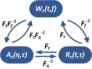
where the kernel function [math]\displaystyle{ \Pi (t,f) }[/math] is defined in the time-frequency domain instead of the ambiguity one. In the original Wigner representation, [math]\displaystyle{ \Pi = \delta_{(0,0)} }[/math]. The relationship between the two kernels is the same as the one between the WD and the AF, namely two successive Fourier transforms (cf. diagram).
- [math]\displaystyle{ \Phi = \mathcal{F}_t \mathcal{F}^{-1}_f \Pi }[/math]
i.e.
- [math]\displaystyle{ \Phi(\eta, \tau) = \int_{-\infty}^\infty \int_{-\infty}^\infty \Pi(t,f) \exp (-j2\pi(t \eta-f \tau))\, dt \, df, }[/math]
or equivalently
- [math]\displaystyle{ \Pi(t,f) = \int_{-\infty}^\infty \int_{-\infty}^\infty \Phi(\eta,\tau) \exp (j2\pi(\eta t-\tau f))\, d\eta \, d\tau. }[/math]
Ambiguity function
The class of bilinear (or quadratic) time–frequency distributions can be most easily understood in terms of the ambiguity function, an explanation of which follows.
Consider the well known power spectral density [math]\displaystyle{ P_x(f) }[/math] and the signal auto-correlation function [math]\displaystyle{ R_x (\tau) }[/math] in the case of a stationary process. The relationship between these functions is as follows:
- [math]\displaystyle{ P_x(f)= \int_{-\infty}^\infty R_x(\tau)e^{-j2\pi f\tau} \, d\tau, }[/math]
- [math]\displaystyle{ R_x(\tau) = \int_{-\infty}^\infty x \left (t+ \tfrac{\tau}{2} \right )x^* \left (t- \tfrac{\tau}{2} \right ) \, dt. }[/math]
For a non-stationary signal [math]\displaystyle{ x(t) }[/math], these relations can be generalized using a time-dependent power spectral density or equivalently the famous Wigner distribution function of [math]\displaystyle{ x(t) }[/math] as follows:
- [math]\displaystyle{ W_x(t, f)= \int_{-\infty}^\infty R_x(t, \tau)e^{-j2\pi f\tau}\, d\tau, }[/math]
- [math]\displaystyle{ R_x (t ,\tau) = x \left (t+ \tfrac{\tau}{2} \right )x^* \left(t- \tfrac{\tau}{2} \right). }[/math]
If the Fourier transform of the auto-correlation function is taken with respect to t instead of τ, we get the ambiguity function as follows:
- [math]\displaystyle{ A_x(\eta,\tau)=\int_{-\infty}^\infty x \left (t+ \tfrac{\tau}{2} \right )x^* \left(t- \tfrac{\tau}{2} \right)e^{j2\pi t\eta}\, dt. }[/math]
The relationship between the Wigner distribution function, the auto-correlation function and the ambiguity function can then be illustrated by the following figure.
By comparing the definition of bilinear (or quadratic) time–frequency distributions with that of the Wigner distribution function, it is easily found that the latter is a special case of the former with [math]\displaystyle{ \Phi(\eta,\tau) = 1 }[/math]. Alternatively, bilinear (or quadratic) time–frequency distributions can be regarded as a masked version of the Wigner distribution function if a kernel function [math]\displaystyle{ \Phi(\eta,\tau) \neq 1 }[/math] is chosen. A properly chosen kernel function can significantly reduce the undesirable cross-term of the Wigner distribution function.
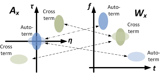
What is the benefit of the additional kernel function? The following figure shows the distribution of the auto-term and the cross-term of a multi-component signal in both the ambiguity and the Wigner distribution function.
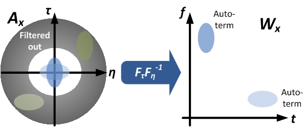
For multi-component signals in general, the distribution of its auto-term and cross-term within its Wigner distribution function is generally not predictable, and hence the cross-term cannot be removed easily. However, as shown in the figure, for the ambiguity function, the auto-term of the multi-component signal will inherently tend to close the origin in the ητ-plane, and the cross-term will tend to be away from the origin. With this property, the cross-term in can be filtered out effortlessly if a proper low-pass kernel function is applied in ητ-domain. The following is an example that demonstrates how the cross-term is filtered out.
Kernel properties
The Fourier transform of [math]\displaystyle{ \theta (u,\xi ) }[/math] is
- [math]\displaystyle{ \hat{\theta}(\tau ,\gamma )=\int_{-\infty }^{\infty} \int_{-\infty }^{\infty} \theta (u,\xi ) e^{-i(u\gamma +\xi \tau )} \, du \, d\xi }[/math]
The following proposition gives necessary and sufficient conditions to ensure that [math]\displaystyle{ P_\theta }[/math] satisfies marginal energy properties like those of the Wigner–Ville distribution.
- Proposition: The marginal energy properties
- [math]\displaystyle{ \int_{-\infty }^\infty P_\theta f(u,\xi ) \, d\xi =2\pi | f(u) |^2, }[/math]
- [math]\displaystyle{ \int_{-\infty }^\infty P_\theta f(u,\xi ) \, du= |\hat{f}(\xi )|^2 }[/math]
- are satisfied for all [math]\displaystyle{ f\in L^2(\mathbf{R}) }[/math] if and only if
- [math]\displaystyle{ \forall (\tau ,\gamma )\in \mathbf{R}^2: \qquad \hat{\theta}(\tau ,0)=\hat{\theta }(0,\gamma )=1 }[/math]
Some time-frequency distributions
Wigner distribution function
Aforementioned, the Wigner distribution function is a member of the class of quadratic time-frequency distributions (QTFDs) with the kernel function [math]\displaystyle{ \Phi (\eta,\tau) = 1 }[/math]. The definition of Wigner distribution is as follows:
- [math]\displaystyle{ W_x(t, f)= \int_{-\infty}^\infty x \left (t+ \tfrac{\tau}{2} \right ) x^*\left(t- \tfrac{\tau}{2} \right)e ^{-j2\pi f\tau}\, d\tau. }[/math]
Modified Wigner distribution functions
Affine invariance
We can design time-frequency energy distributions that satisfy the scaling property
- [math]\displaystyle{ \frac{1}{\sqrt{s}}f\left( \tfrac{t}{s} \right) \longleftrightarrow P_V f\left( \tfrac{u}{s},s\xi \right) }[/math]
as does the Wigner–Ville distribution. If
- [math]\displaystyle{ g(t)=\frac{1}{\sqrt{s}}f\left( \tfrac{t}{s} \right) }[/math]
then
- [math]\displaystyle{ P_\theta g(u,\xi)= P_\theta f\left( \tfrac{u}{s},s\xi \right). }[/math]
This is equivalent to imposing that
- [math]\displaystyle{ \forall s\in \mathbf{R}^+: \qquad \theta \left( su,\tfrac{\xi }{s} \right)=\theta (u,\xi) , }[/math]
and hence
- [math]\displaystyle{ \theta (u,\xi )=\theta (u\xi ,1)=\beta (u\xi ) }[/math]
The Rihaczek and Choi–Williams distributions are examples of affine invariant Cohen's class distributions.
Choi–Williams distribution function
The kernel of Choi–Williams distribution is defined as follows:
- [math]\displaystyle{ \Phi (\eta,\tau ) = \exp (-\alpha(\eta \tau)^2), }[/math]
where α is an adjustable parameter.
Rihaczek distribution function
The kernel of Rihaczek distribution is defined as follows:
- [math]\displaystyle{ \Phi (\eta,\tau) = \exp \left(-i 2\pi \frac{\eta \tau}{2} \right), }[/math]
With this particular kernel a simple calculation proves that
- [math]\displaystyle{ C_x (t,f) = x(t) \hat{x}^*(f) e^{i 2\pi t f} }[/math]
Cone-shape distribution function
The kernel of cone-shape distribution function is defined as follows:
- [math]\displaystyle{ \Phi (\eta,\tau) = \frac{\sin(\pi \eta \tau)}{ \pi \eta \tau }\exp \left(-2\pi \alpha \tau^2 \right), }[/math]
where α is an adjustable parameter. See Transformation between distributions in time-frequency analysis. More such QTFDs and a full list can be found in, e.g., Cohen's text cited.
Spectrum of non-stationary processes
A time-varying spectrum for non-stationary processes is defined from the expected Wigner–Ville distribution. Locally stationary processes appear in many physical systems where random fluctuations are produced by a mechanism that changes slowly in time. Such processes can be approximated locally by a stationary process. Let [math]\displaystyle{ X(t) }[/math] be a real valued zero-mean process with covariance
- [math]\displaystyle{ R(t,s)=E[X(t)X(s)] }[/math]
The covariance operator K is defined for any deterministic signal [math]\displaystyle{ f\in L^2(\mathbf{R}) }[/math] by
- [math]\displaystyle{ Kf(t)=\int_{-\infty}^\infty R( t,s)f(s) \, ds }[/math]
For locally stationary processes, the eigenvectors of K are well approximated by the Wigner–Ville spectrum.
Wigner–Ville spectrum
The properties of the covariance [math]\displaystyle{ R(t,s) }[/math] are studied as a function of [math]\displaystyle{ \tau =t-s }[/math] and [math]\displaystyle{ u=\frac{t+s}{2} }[/math]:
- [math]\displaystyle{ R(t,s)=R\left( u+\tfrac{\tau }{2},u-\tfrac{\tau}{2} \right)=C( u,\tau) }[/math]
The process is wide-sense stationary if the covariance depends only on [math]\displaystyle{ \tau =t-s }[/math]:
- [math]\displaystyle{ Kf(t)=\int_{-\infty}^\infty C(t-s) f(s)\,ds=C*f(t) }[/math]
The eigenvectors are the complex exponentials [math]\displaystyle{ e^{i\omega t} }[/math] and the corresponding eigenvalues are given by the power spectrum
- [math]\displaystyle{ P_X (\omega)=\int_{-\infty }^\infty C(\tau) e^{-i\omega \tau } \, d\tau }[/math]
For non-stationary processes, Martin and Flandrin have introduced a time-varying spectrum
- [math]\displaystyle{ P_X ( u,\xi)=\int_{-\infty }^\infty C(u,\tau) e^{-i\xi \tau} \, d\tau =\int_{-\infty}^\infty E\left [ X\left( u+\tfrac{\tau}{2} \right) X\left( u-\tfrac{\tau}{2} \right) \right ] e^{-i\xi \tau } \, d\tau }[/math]
To avoid convergence issues we suppose that X has compact support so that [math]\displaystyle{ C(u,\tau) }[/math] has compact support in [math]\displaystyle{ \tau }[/math]. From above we can write
- [math]\displaystyle{ P_X ( u,\xi)=E[ P_V X ( u,\xi)] }[/math]
which proves that the time varying spectrum is the expected value of the Wigner–Ville transform of the process X. Here, the Wigner–Ville stochastic integral is interpreted as a mean-square integral:[2]
- [math]\displaystyle{ P_V ( u,\xi)=\int_{-\infty}^\infty \left\{ X\left( u+\tfrac{\tau}{2}\right)X\left( u-\tfrac{\tau }{2} \right) \right\} e^{-i\xi \tau} \, d\tau }[/math]
References
- L. Cohen, Time-Frequency Analysis, Prentice-Hall, New York, 1995. ISBN:978-0135945322
- B. Boashash, editor, “Time-Frequency Signal Analysis and Processing – A Comprehensive Reference”, Elsevier Science, Oxford, 2003.
- L. Cohen, “Time-Frequency Distributions—A Review,” Proceedings of the IEEE, vol. 77, no. 7, pp. 941–981, 1989.
- S. Qian and D. Chen, Joint Time-Frequency Analysis: Methods and Applications, Chap. 5, Prentice Hall, N.J., 1996.
- H. Choi and W. J. Williams, “Improved time-frequency representation of multicomponent signals using exponential kernels,” IEEE. Trans. Acoustics, Speech, Signal Processing, vol. 37, no. 6, pp. 862–871, June 1989.
- Y. Zhao, L. E. Atlas, and R. J. Marks, “The use of cone-shape kernels for generalized time-frequency representations of nonstationary signals,” IEEE Trans. Acoustics, Speech, Signal Processing, vol. 38, no. 7, pp. 1084–1091, July 1990.
- B. Boashash, “Heuristic Formulation of Time-Frequency Distributions”, Chapter 2, pp. 29–58, in B. Boashash, editor, Time-Frequency Signal Analysis and Processing: A Comprehensive Reference, Elsevier Science, Oxford, 2003.
- B. Boashash, “Theory of Quadratic TFDs”, Chapter 3, pp. 59–82, in B. Boashash, editor, Time-Frequency Signal Analysis & Processing: A Comprehensive Reference, Elsevier, Oxford, 2003.
 |


