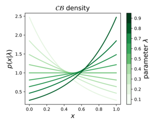
Continuous Bernoulli distribution
|
Probability density function  | |||
| Notation | [math]\displaystyle{ \mathcal{CB}(\lambda) }[/math] | ||
|---|---|---|---|
| Parameters | [math]\displaystyle{ \lambda \in (0,1) }[/math] | ||
| Support | [math]\displaystyle{ x \in [0, 1] }[/math] | ||
|
[math]\displaystyle{ C(\lambda) \lambda^x (1-\lambda)^{1-x}\! }[/math] where [math]\displaystyle{ C(\lambda) = \begin{cases} 2 &\text{if } \lambda = \frac{1}{2}\\ \frac{2 \tanh^{-1}(1-2\lambda)}{1-2\lambda} &\text{ otherwise} \end{cases} }[/math] | |||
| CDF | [math]\displaystyle{ \begin{cases} x &\text{ if } \lambda = \frac{1}{2} \\ \frac{\lambda^x (1-\lambda)^{1-x} + \lambda - 1}{2\lambda - 1} &\text{ otherwise} \end{cases}\! }[/math] | ||
| Mean | [math]\displaystyle{ \operatorname{E}[X] = \begin{cases} \frac{1}{2} &\text{ if } \lambda = \frac{1}{2} \\ \frac{\lambda}{2\lambda - 1} + \frac{1}{2 \tanh^{-1}(1-2\lambda)} &\text{ otherwise} \end{cases}\! }[/math] | ||
| Variance | [math]\displaystyle{ \operatorname{var}[X] = \begin{cases} \frac{1}{12} &\text{ if } \lambda = \frac{1}{2} \\ -\frac{(1-\lambda) \lambda}{(1-2\lambda)^2} + \frac{1}{(2 \tanh^{-1}(1-2\lambda))^2} &\text{ otherwise} \end{cases}\! }[/math] | ||
In probability theory, statistics, and machine learning, the continuous Bernoulli distribution[1][2][3] is a family of continuous probability distributions parameterized by a single shape parameter [math]\displaystyle{ \lambda \in (0, 1) }[/math], defined on the unit interval [math]\displaystyle{ x \in [0, 1] }[/math], by:
- [math]\displaystyle{ p(x | \lambda) \propto \lambda^x (1-\lambda)^{1-x}. }[/math]
The continuous Bernoulli distribution arises in deep learning and computer vision, specifically in the context of variational autoencoders,[4][5] for modeling the pixel intensities of natural images. As such, it defines a proper probabilistic counterpart for the commonly used binary cross entropy loss, which is often applied to continuous, [math]\displaystyle{ [0,1] }[/math]-valued data.[6][7][8][9] This practice amounts to ignoring the normalizing constant of the continuous Bernoulli distribution, since the binary cross entropy loss only defines a true log-likelihood for discrete, [math]\displaystyle{ \{0,1\} }[/math]-valued data.
The continuous Bernoulli also defines an exponential family of distributions. Writing [math]\displaystyle{ \eta = \log\left(\lambda/(1-\lambda)\right) }[/math] for the natural parameter, the density can be rewritten in canonical form: [math]\displaystyle{ p(x | \eta) \propto \exp (\eta x) }[/math].
Related distributions
Bernoulli distribution
The continuous Bernoulli can be thought of as a continuous relaxation of the Bernoulli distribution, which is defined on the discrete set [math]\displaystyle{ \{0,1\} }[/math] by the probability mass function:
- [math]\displaystyle{ p(x) = p^x (1-p)^{1-x}, }[/math]
where [math]\displaystyle{ p }[/math] is a scalar parameter between 0 and 1. Applying this same functional form on the continuous interval [math]\displaystyle{ [0,1] }[/math] results in the continuous Bernoulli probability density function, up to a normalizing constant.
Beta distribution
The Beta distribution has the density function:
- [math]\displaystyle{ p(x) \propto x^{\alpha - 1} (1-x)^{\beta - 1}, }[/math]
which can be re-written as:
- [math]\displaystyle{ p(x) \propto x_1^{\alpha_1 - 1} x_2^{\alpha_2 - 1}, }[/math]
where [math]\displaystyle{ \alpha_1, \alpha_2 }[/math] are positive scalar parameters, and [math]\displaystyle{ (x_1, x_2) }[/math] represents an arbitrary point inside the 1-simplex, [math]\displaystyle{ \Delta^{1} = \{ (x_1, x_2): x_1 \gt 0, x_2 \gt 0, x_1 + x_2 = 1 \} }[/math]. Switching the role of the parameter and the argument in this density function, we obtain:
- [math]\displaystyle{ p(x) \propto \alpha_1^{x_1} \alpha_2^{x_2}. }[/math]
This family is only identifiable up to the linear constraint [math]\displaystyle{ \alpha_1 + \alpha_2 = 1 }[/math], whence we obtain:
- [math]\displaystyle{ p(x) \propto \lambda^{x_1} (1-\lambda)^{x_2}, }[/math]
corresponding exactly to the continuous Bernoulli density.
Exponential distribution
An exponential distribution restricted to the unit interval is equivalent to a continuous Bernoulli distribution with appropriate[which?] parameter.
Continuous categorical distribution
The multivariate generalization of the continuous Bernoulli is called the continuous-categorical.[10]
References
- ↑ Loaiza-Ganem, G., & Cunningham, J. P. (2019). The continuous Bernoulli: fixing a pervasive error in variational autoencoders. In Advances in Neural Information Processing Systems (pp. 13266-13276).
- ↑ PyTorch Distributions. https://pytorch.org/docs/stable/distributions.html#continuousbernoulli
- ↑ Tensorflow Probability. https://www.tensorflow.org/probability/api_docs/python/tfp/edward2/ContinuousBernoulli
- ↑ Kingma, D. P., & Welling, M. (2013). Auto-encoding variational bayes. arXiv preprint arXiv:1312.6114.
- ↑ Kingma, D. P., & Welling, M. (2014, April). Stochastic gradient VB and the variational auto-encoder. In Second International Conference on Learning Representations, ICLR (Vol. 19).
- ↑ Larsen, A. B. L., Sønderby, S. K., Larochelle, H., & Winther, O. (2016, June). Autoencoding beyond pixels using a learned similarity metric. In International conference on machine learning (pp. 1558-1566).
- ↑ Jiang, Z., Zheng, Y., Tan, H., Tang, B., & Zhou, H. (2017, August). Variational deep embedding: an unsupervised and generative approach to clustering. In Proceedings of the 26th International Joint Conference on Artificial Intelligence (pp. 1965-1972).
- ↑ PyTorch VAE tutorial: https://github.com/pytorch/examples/tree/master/vae.
- ↑ Keras VAE tutorial: https://blog.keras.io/building-autoencoders-in-keras.html.
- ↑ Gordon-Rodriguez, E., Loaiza-Ganem, G., & Cunningham, J. P. (2020). The continuous categorical: a novel simplex-valued exponential family. In 36th International Conference on Machine Learning, ICML 2020. International Machine Learning Society (IMLS).
 |

