Information dimension
In information theory, information dimension is an information measure for random vectors in Euclidean space, based on the normalized entropy of finely quantized versions of the random vectors. This concept was first introduced by Alfréd Rényi in 1959.[1]
Simply speaking, it is a measure of the fractal dimension of a probability distribution. It characterizes the growth rate of the Shannon entropy given by successively finer discretizations of the space.
In 2010, Wu and Verdú gave an operational characterization of Rényi information dimension as the fundamental limit of almost lossless data compression for analog sources under various regularity constraints of the encoder/decoder.
Definition and Properties
The entropy of a discrete random variable [math]\displaystyle{ Z }[/math] is
- [math]\displaystyle{ \mathbb{H}_0(Z)=\sum_{z \in supp(P_Z)}P_Z(z)\log_2\frac{1}{P_Z(z)} }[/math]
where [math]\displaystyle{ P_Z(z) }[/math] is the probability measure of [math]\displaystyle{ Z }[/math] when [math]\displaystyle{ Z=z }[/math], and the [math]\displaystyle{ supp(P_Z) }[/math] denotes a set [math]\displaystyle{ \{z|z \in\mathcal{Z},P_Z(z)\gt 0\} }[/math].
Let [math]\displaystyle{ X }[/math] be an arbitrary real-valued random variable. Given a positive integer [math]\displaystyle{ m }[/math], we create a new discrete random variable
- [math]\displaystyle{ \langle X\rangle_m=\frac{\lfloor mX\rfloor}{m} }[/math]
where the [math]\displaystyle{ \lfloor \cdot \rfloor }[/math] is the floor operator which converts a real number to the greatest integer less than it. Then
- [math]\displaystyle{ \underline{d}(X)=\liminf_{m \rightarrow \infty}\frac{\mathbb{H}_0(\langle X \rangle_m)}{\log_2m} }[/math]
and
- [math]\displaystyle{ \bar{d}(X)=\limsup_{m \rightarrow \infty}\frac{\mathbb{H}_0(\langle X \rangle_m)}{\log_2m} }[/math]
are called lower and upper information dimensions of [math]\displaystyle{ X }[/math] respectively. When [math]\displaystyle{ \underline{d}(X)=\bar{d}(X) }[/math], we call this value information dimension of [math]\displaystyle{ X }[/math],
- [math]\displaystyle{ d(X)=\lim_{m \rightarrow \infty}\frac{\mathbb{H}_0(\langle X \rangle_m)}{\log_2m} }[/math]
Some important properties of information dimension [math]\displaystyle{ d(X) }[/math]:
- If the mild condition [math]\displaystyle{ \mathbb{H}(\lfloor X\rfloor)\lt \infty }[/math] is fulfilled, we have [math]\displaystyle{ 0\leq\underline{d}(X)\leq\bar{d}(X)\leq1 }[/math].
- For an [math]\displaystyle{ n }[/math]-dimensional random vector [math]\displaystyle{ \vec{X} }[/math], the first property can be generalized to [math]\displaystyle{ 0\leq\underline{d}(\vec{X})\leq \bar{d}(\vec{X})\leq n }[/math].
- It is sufficient to calculate the upper and lower information dimensions when restricting to the exponential subsequence [math]\displaystyle{ m=2^l }[/math].
- [math]\displaystyle{ \underline{d}(X) }[/math] and [math]\displaystyle{ \bar{d}(X) }[/math] are kept unchanged if rounding or ceiling functions are used in quantization.
d-Dimensional Entropy
If the information dimension [math]\displaystyle{ d }[/math] exists, one can define the [math]\displaystyle{ d }[/math]-dimensional entropy of this distribution by
- [math]\displaystyle{ \mathbb{H}_{d(X)}(X)=\lim_{n \rightarrow + \infty}(\mathbb{H}_0(\langle X \rangle_n)-d(X)\log_2n) }[/math]
provided the limit exists. If [math]\displaystyle{ d=0 }[/math], the zero-dimensional entropy equals the standard Shannon entropy [math]\displaystyle{ \mathbb{H}_0(X) }[/math]. For integer dimension [math]\displaystyle{ d=n\ge 1 }[/math], the [math]\displaystyle{ n }[/math]-dimensional entropy is the [math]\displaystyle{ n }[/math]-fold integral defining the respective differential entropy.
An equivalent definition of Information Dimension
In 1994, Kawabata and Dembo in Kawabata & Dembo 1994 proposed a new way of measuring information based on rate distortion value of a random variable. The measure is defined as
- [math]\displaystyle{ d_R(X)=-2\frac{R(X, D)}{\log D}, }[/math]
where [math]\displaystyle{ R(X, D) }[/math] is the rate-distortion function that is defined as
- [math]\displaystyle{ R(X, D) = \min_{\|X-\hat{X}\|_2\leq D} I(X, \hat{X}), }[/math]
or equivalently, minimum information that could lead to a [math]\displaystyle{ D }[/math]-close approximation of [math]\displaystyle{ X }[/math].
They further, proved that such definition is equivalent to the definition of information dimension. Formally,
- [math]\displaystyle{ d_R(X) = d(X). }[/math]
Dimensional-Rate Bias
Using the above definition of Rényi information dimension, a similar measure to d-dimensional entropy is defined in Charusaie, Amini & Rini 2022 . This value [math]\displaystyle{ b(X) }[/math] that is named dimensional-rate bias is defined in a way to capture the finite term of rate-distortion function. Formally,
- [math]\displaystyle{ R(X, D)=-\frac{d(X)}{2}\log \frac{2\pi e D}{d(X)}+b(X). }[/math]
The dimensional-rate bias is equal to d-dimensional rate for continuous, discrete, and discrete-continuous mixed distribution. Furthermore, it is calculable for a set of singular random variables, while d-dimensional entropy does not necessarily exist there.
Finally, dimensional-rate bias generalizes the Shannon's entropy and differential entropy, as one could find the mutual information [math]\displaystyle{ I(X; Y) }[/math] using the following formula:
- [math]\displaystyle{ I(X;Y) = b(X)+b(Y)-b(X, Y). }[/math]
Discrete-Continuous Mixture Distributions
According to Lebesgue decomposition theorem,[2] a probability distribution can be uniquely represented by the mixture
[math]\displaystyle{ v=pP_{Xd}+qP_{Xc}+rP_{Xs} }[/math]
where [math]\displaystyle{ p+q+r=1 }[/math] and [math]\displaystyle{ p,q,r\geq0 }[/math]; [math]\displaystyle{ P_{Xd} }[/math] is a purely atomic probability measure (discrete part), [math]\displaystyle{ P_{Xc} }[/math] is the absolutely continuous probability measure, and [math]\displaystyle{ P_{Xs} }[/math] is a probability measure singular with respect to Lebesgue measure but with no atoms (singular part). Let [math]\displaystyle{ X }[/math] be a random variable such that [math]\displaystyle{ \mathbb{H}(\lfloor X \rfloor) \lt \infty }[/math]. Assume the distribution of [math]\displaystyle{ X }[/math] can be represented as
[math]\displaystyle{ v=(1-\rho)P_{Xd}+\rho P_{Xc} }[/math]
where [math]\displaystyle{ P_{Xd} }[/math] is a discrete measure and [math]\displaystyle{ P_{Xc} }[/math] is the absolutely continuous probability measure with [math]\displaystyle{ 0\leq\rho\leq1 }[/math]. Then
[math]\displaystyle{ d(X)=\rho }[/math]
Moreover, given [math]\displaystyle{ \mathbb{H}_0(P_{Xd}) }[/math] and differential entropy [math]\displaystyle{ h(P_{Xc}) }[/math], the [math]\displaystyle{ d }[/math]-Dimensional Entropy is simply given by
[math]\displaystyle{ \mathbb{H}_\rho(X)=(1-\rho)\mathbb{H}_0(P_{Xd})+\rho h(P_{Xc})+\mathbb{H}_0(\rho) }[/math]
where [math]\displaystyle{ \mathbb{H}_0(\rho) }[/math] is the Shannon entropy of a discrete random variable [math]\displaystyle{ Z }[/math] with [math]\displaystyle{ P_Z(1)=\rho }[/math] and [math]\displaystyle{ P_Z(0)=1-\rho }[/math] and given by
[math]\displaystyle{ \mathbb{H}_0(\rho)=\rho\log_2\frac{1}{\rho}+(1-\rho)\log_2\frac{1}{1-\rho} }[/math]
Example
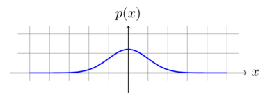
Consider a signal which has a Gaussian probability distribution.
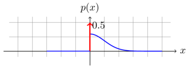
We pass the signal through a half-wave rectifier which converts all negative value to 0, and maintains all other values. The half-wave rectifier can be characterized by the function
[math]\displaystyle{ f(x)= \begin{cases} x,& \text{if } x\geq 0\\ 0,&x\lt 0 \end{cases} }[/math]
Then, at the output of the rectifier, the signal has a rectified Gaussian distribution. It is characterized by an atomic mass of weight 0.5 and has a Gaussian PDF for all [math]\displaystyle{ x\gt 0 }[/math].
With this mixture distribution, we apply the formula above and get the information dimension [math]\displaystyle{ d }[/math] of the distribution and calculate the [math]\displaystyle{ d }[/math]-dimensional entropy.
[math]\displaystyle{ d(X)=\rho=0.5 }[/math]
The normalized right part of the zero-mean Gaussian distribution has entropy [math]\displaystyle{ h(P_{Xc})=\frac{1}{2}\log_2(2\pi e\sigma^2)-1 }[/math], hence
[math]\displaystyle{ \begin{align} \mathbb{H}_{0.5}(X)&=(1-0.5)(1\log_21)+0.5h(P_{Xc})+\mathbb{H}_0(0.5)\\ &=0+\frac{1}{2}(\frac{1}{2}\log_2(2\pi e\sigma^2)-1)+1\\ &=\frac{1}{4}\log_2(2\pi e\sigma^2)+\frac{1}{2}\,\text{ bit(s)} \end{align} }[/math]
Connection to Differential Entropy
It is shown [3] that information dimension and differential entropy are tightly connected.
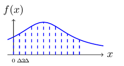
Let [math]\displaystyle{ X }[/math] be a random variable with continuous density [math]\displaystyle{ f(x) }[/math].
Suppose we divide the range of [math]\displaystyle{ X }[/math] into bins of length [math]\displaystyle{ \Delta }[/math]. By the mean value theorem, there exists a value [math]\displaystyle{ x_i }[/math] within each bin such that
- [math]\displaystyle{ f(x_i)\Delta=\int_{i\Delta}^{(i+1)\Delta}f(x)\;\mathrm{d}x }[/math]
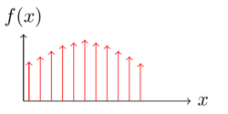
Consider the discretized random variable [math]\displaystyle{ X^\Delta=x_i }[/math] if [math]\displaystyle{ i\Delta\leq X\lt (i+1)\Delta }[/math].
The probability of each support point [math]\displaystyle{ X^\Delta=x_i }[/math] is
- [math]\displaystyle{ P_{X^\Delta}(x_i)=\int_{i\Delta}^{(i+1)\Delta}f(x)\;\mathrm{d}x=f(x_i)\Delta }[/math]
Let [math]\displaystyle{ S = \operatorname{supp}(P_{X^\Delta}) }[/math]. The entropy of [math]\displaystyle{ X^\Delta }[/math] is
- [math]\displaystyle{ \begin{align} \mathbb{H}_0(X^\Delta)&=-\sum_{x_i \in S} P_{X^\Delta}\log_2P_{X^\Delta}\\ &=-\sum_{x_i \in S} f(x_i)\Delta\log_2(f(x_i)\Delta)\\ &=-\sum_{x_i \in S} \Delta f(x_i)\log_2f(x_i)-\sum_{x_i \in S} f(x_i)\Delta \log_2\Delta\\ &=-\sum_{x_i \in S} \Delta f(x_i)\log_2f(x_i)-\log_2\Delta\\ \end{align} }[/math]
If we set [math]\displaystyle{ \Delta=1/m }[/math] and [math]\displaystyle{ x_i=i/m }[/math] then we are doing exactly the same quantization as the definition of information dimension. Since relabeling the events of a discrete random variable does not change its entropy, we have
- [math]\displaystyle{ \mathbb{H}_0(X^{1/m})=\mathbb{H}_0(\langle X\rangle_m). }[/math]
This yields
- [math]\displaystyle{ \mathbb{H}_0(\langle X\rangle_m)=-\sum \frac{1}{m} f(x_i)\log_2f(x_i)+\log_2m }[/math]
and when [math]\displaystyle{ m }[/math] is sufficiently large,
- [math]\displaystyle{ -\sum \Delta f(x_i)\log_2f(x_i) \approx \int f(x)\log_2 \frac{1}{f(x)}\mathrm{d}x }[/math]
which is the differential entropy [math]\displaystyle{ h(x) }[/math] of the continuous random variable. In particular, if [math]\displaystyle{ f(x) }[/math] is Riemann integrable, then
- [math]\displaystyle{ h(X)=\lim_{m\rightarrow \infty}\mathbb{H}_0(\langle X\rangle_m)-\log_2(m). }[/math]
Comparing this with the [math]\displaystyle{ d }[/math]-dimensional entropy shows that the differential entropy is exactly the one-dimensional entropy
- [math]\displaystyle{ h(X)=\mathbb{H}_1(X). }[/math]
In fact, this can be generalized to higher dimensions. Rényi shows that, if [math]\displaystyle{ \vec{X} }[/math] is a random vector in a [math]\displaystyle{ n }[/math]-dimensional Euclidean space [math]\displaystyle{ \real^n }[/math] with an absolutely continuous distribution with a probability density function [math]\displaystyle{ f_{\vec{X}}(\vec{x}) }[/math] and finite entropy of the integer part ([math]\displaystyle{ H_0(\langle \vec{X} \rangle_m)\lt \infty }[/math]), we have [math]\displaystyle{ d(\vec{X})=n }[/math]
and
- [math]\displaystyle{ \mathbb{H}_n(\vec{X})=\int\cdots\int f_{\vec{X}}(\vec{x})\log_2\frac{1}{f_{\vec{X}}(\vec{x})}\mathrm{d}\vec{x}, }[/math]
if the integral exists.
Lossless data compression
The information dimension of a distribution gives a theoretical upper bound on the compression rate, if one wants to compress a variable coming from this distribution. In the context of lossless data compression, we try to compress real number with less real number which both have infinite precision.
The main objective of the lossless data compression is to find efficient representations for source realizations [math]\displaystyle{ x^n\in \mathcal{X}^n }[/math] by [math]\displaystyle{ y^n\in\mathcal{Y}^n }[/math]. A [math]\displaystyle{ (n,k)- }[/math]code for [math]\displaystyle{ \{X_i:i\in\mathcal{N}\} }[/math] is a pair of mappings:
- encoder: [math]\displaystyle{ f_n:\mathcal{X}^n\rightarrow \mathcal{Y}^k }[/math] which converts information from a source into symbols for communication or storage;
- decoder: [math]\displaystyle{ g_n:\mathcal{Y}^k\rightarrow\mathcal{X}^n }[/math] is the reverse process, converting code symbols back into a form that the recipient understands.
The block error probability is [math]\displaystyle{ \mathcal{P}\{g_n(f_n(X^n))\neq X^n\} }[/math].
Define [math]\displaystyle{ r(\epsilon) }[/math] to be the infimum of [math]\displaystyle{ r\geq0 }[/math] such that there exists a sequence of [math]\displaystyle{ (n,\lfloor rn\rfloor)- }[/math]codes such that [math]\displaystyle{ \mathcal{P}\{g_n(f_n(X^n))\neq X^n\}\leq\epsilon }[/math] for all sufficiently large [math]\displaystyle{ n }[/math].
So [math]\displaystyle{ r(\epsilon) }[/math] basically gives the ratio between the code length and the source length, it shows how good a specific encoder decoder pair is. The fundamental limits in lossless source coding are as follows.[4]
Consider a continuous encoder function [math]\displaystyle{ f(x):\real^n\rightarrow \real^{\lfloor Rn\rfloor} }[/math] with its continuous decoder function [math]\displaystyle{ g(x):\real^{\lfloor Rn\rfloor}\rightarrow \real^n }[/math]. If we impose no regularity on [math]\displaystyle{ f(x) }[/math] and [math]\displaystyle{ g(x) }[/math], due to the rich structure of [math]\displaystyle{ \real }[/math], we have the minimum [math]\displaystyle{ \epsilon }[/math]-achievable rate [math]\displaystyle{ R_0(\epsilon)=0 }[/math] for all [math]\displaystyle{ 0\lt \epsilon\leq1 }[/math]. It means that one can build an encoder-decoder pair with infinity compression rate.
In order to get some nontrivial and meaningful conclusions, let [math]\displaystyle{ R^*(\epsilon ) }[/math] the minimum [math]\displaystyle{ \epsilon- }[/math]achievable rate for linear encoder and Borel decoder. If random variable [math]\displaystyle{ X }[/math] has a distribution which is a mixture of discrete and continuous part. Then [math]\displaystyle{ R^*(\epsilon)=d(X) }[/math] for all [math]\displaystyle{ 0\lt \epsilon\leq1 }[/math] Suppose we restrict the decoder to be a Lipschitz continuous function and [math]\displaystyle{ \bar{d}(X)\lt \infty }[/math] holds, then the minimum [math]\displaystyle{ \epsilon- }[/math]achievable rate [math]\displaystyle{ R(\epsilon)\geq \bar{d}(X) }[/math] for all [math]\displaystyle{ 0\lt \epsilon\leq1 }[/math].
The fundamental role of information dimension in lossless data compression further extends beyond the i.i.d. data. It is shown that for specified processes (e.g., moving-average processes) the ratio of lossless compression is also equal to the information dimension rate rate.[5] This result allows for further compression that was not possible by considering only marginal distribution of the process.
See also
Notes
- ↑ See Rényi 1959.
- ↑ See Çınlar 2011.
- ↑ See Cover & Thomas 2012.
- ↑ See Wu & Verdu 2010.
- ↑ See Charusaie, Amini & Rini 2022
References
- Çınlar, Erhan (2011). Probability and Stochastics. Graduate Texts in Mathematics. 261. Springer. doi:10.1007/978-0-387-87859-1. ISBN 978-0-387-87858-4.
- Cover, Thomas M.; Thomas, Joy A. (2012). Elements of Information Theory (2nd ed.). Wiley. pp. 247–248. ISBN 9781118585771. https://books.google.com/books?id=VWq5GG6ycxMC.
- Rényi, A. (March 1959). "On the dimension and entropy of probability distributions". Acta Mathematica Academiae Scientiarum Hungaricae 10 (1–2): 193–215. doi:10.1007/BF02063299. ISSN 0001-5954.
- Wu, Yihong; Verdu, S. (August 2010). "Rényi Information Dimension: Fundamental Limits of Almost Lossless Analog Compression". IEEE Transactions on Information Theory 56 (8): 3721–3748. doi:10.1109/TIT.2010.2050803. ISSN 0018-9448.
- Charusaie, M.; Amini, A.; Rini, S. (May 2022). "Compressibility Measures for Affinely Singular Random Vectors". IEEE Transactions on Information Theory: 1–1. doi:10.1109/TIT.2022.3174623.
- Kawabata, T.; Dembo, A. (September 1994). "The Rate-Distortion Dimension of Sets and Measures". IEEE Transactions on Information Theory: 1–1. doi:10.1109/18.333868.
 |


