Chow test

Short description: Mathematical test proposed by Gregory Chow

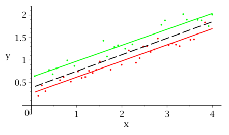
The Chow test (Chinese: 鄒檢定), proposed by econometrician Gregory Chow in 1960, is a test of whether the true coefficients in two linear regressions on different data sets are equal. In econometrics, it is most commonly used in time series analysis to test for the presence of a structural break at a period which can be assumed to be known a priori (for instance, a major historical event such as a war). In program evaluation, the Chow test is often used to determine whether the independent variables have different impacts on different subgroups of the population.

Illustrations

Applications of the Chow test

Structural break (slopes differ)	Program evaluation (intercepts differ)
At [math]\displaystyle{ x=1.7 }[/math] there is a structural break; separate regressions on the subintervals [math]\displaystyle{ [0,1.7] }[/math] and [math]\displaystyle{ [1.7,4] }[/math] delivers a better model than the combined regression (dashed) over the whole interval.	Comparison of two different programs (red, green) in a common data set: separate regressions for both programs deliver a better model than a combined regression (black).

First Chow Test

Suppose that we model our data as

[math]\displaystyle{ y_t=a+bx_{1t} + cx_{2t} + \varepsilon.\, }[/math]

If we split our data into two groups, then we have

[math]\displaystyle{ y_t=a_1+b_1x_{1t} + c_1x_{2t} + \varepsilon \, }[/math]

and

[math]\displaystyle{ y_t=a_2+b_2x_{1t} + c_2x_{2t} + \varepsilon. \, }[/math]

The null hypothesis of the Chow test asserts that [math]\displaystyle{ a_1=a_2 }[/math], [math]\displaystyle{ b_1=b_2 }[/math], and [math]\displaystyle{ c_1=c_2 }[/math], and there is the assumption that the model errors [math]\displaystyle{ \varepsilon }[/math] are independent and identically distributed from a normal distribution with unknown variance.

Let [math]\displaystyle{ S_C }[/math] be the sum of squared residuals from the combined data, [math]\displaystyle{ S_1 }[/math] be the sum of squared residuals from the first group, and [math]\displaystyle{ S_2 }[/math] be the sum of squared residuals from the second group. [math]\displaystyle{ N_1 }[/math] and [math]\displaystyle{ N_2 }[/math] are the number of observations in each group and [math]\displaystyle{ k }[/math] is the total number of parameters (in this case 3, i.e. 2 independent variables coefficients + intercept). Then the Chow test statistic is

[math]\displaystyle{ \frac{(S_C -(S_1+S_2))/k}{(S_1+S_2)/(N_1+N_2-2k)}. }[/math]

The test statistic follows the F-distribution with [math]\displaystyle{ k }[/math] and [math]\displaystyle{ N_1+N_2-2k }[/math] degrees of freedom.

The same result can be achieved via dummy variables.

Consider the two data sets which are being compared. Firstly there is the 'primary' data set i={1,...,[math]\displaystyle{ n_1 }[/math]} and the 'secondary' data set i={[math]\displaystyle{ n_1 }[/math]+1,...,n}. Then there is the union of these two sets: i={1,...,n}. If there is no structural change between the primary and secondary data sets a regression can be run over the union without the issue of biased estimators arising.

Consider the regression:

[math]\displaystyle{ y_t=\beta_0+\beta_1x_{1t} + \beta_2x_{2t} + ... + \beta_kx_{kt} + \gamma_0D_t + \sum_{i=1}^k\gamma_ix_{it}D_t + \varepsilon_t.\, }[/math]

Which is run over i={1,...,n}.

D is a dummy variable taking a value of 1 for i={[math]\displaystyle{ n_1 }[/math]+1,...,n} and 0 otherwise.

If both data sets can be explained fully by [math]\displaystyle{ (\beta_0,\beta_1,...,\beta_k) }[/math] then there is no use in the dummy variable as the data set is explained fully by the restricted equation. That is, under the assumption of no structural change we have a null and alternative hypothesis of:

[math]\displaystyle{ H_0: \gamma_0=0,\gamma_1=0,...,\gamma_k=0 }[/math]

[math]\displaystyle{ H_1: \text{otherwise} }[/math]

The null hypothesis of joint insignificance of D can be run as an F-test with [math]\displaystyle{ n-2(k+1) }[/math] degrees of freedom (DoF). That is: [math]\displaystyle{ F=\frac{(RSS^R-RSS^U)/(k+1)}{RSS^U/DoF} }[/math].

Remarks

• The global sum of squares (SSE) is often called the Restricted Sum of Squares (RSSM) as we basically test a constrained model where we have [math]\displaystyle{ 2k }[/math] assumptions (with [math]\displaystyle{ k }[/math] the number of regressors).
• Some software like SAS will use a predictive Chow test when the size of a subsample is less than the number of regressors.

References

• Chow, Gregory C. (1960). "Tests of Equality Between Sets of Coefficients in Two Linear Regressions". Econometrica 28 (3): 591–605. doi:10.2307/1910133. http://pdfs.semanticscholar.org/0f70/219160c8ad2f9db02e226d3f7d7320e729b8.pdf. 
• Doran, Howard E. (1989). Applied Regression Analysis in Econometrics. CRC Press. p. 146. ISBN 978-0-8247-8049-4. 
• Dougherty, Christopher (2007). Introduction to Econometrics. Oxford University Press. p. 194. ISBN 978-0-19-928096-4. 
• Kmenta, Jan (1986). Elements of Econometrics (Second ed.). New York: Macmillan. pp. 412–423. ISBN 978-0-472-10886-2. https://archive.org/details/elementsofeconom0003kmen. 
• Wooldridge, Jeffrey M. (2009). Introduction to Econometrics: A Modern Approach (Fourth ed.). Mason: South-Western. pp. 243–246. ISBN 978-0-324-66054-8. 

External links

• Computing the Chow statistic, Chow and Wald tests, Chow tests: Series of FAQ explanations from the Stata Corporation at https://www.stata.com/support/faqs/
• [1]: Series of FAQ explanations from the SAS Corporation