Arcsine distribution

Short description: Type of probability distribution

Arcsine

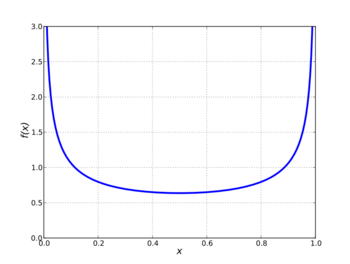
Probability density function
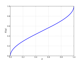
Cumulative distribution function
Parameters	none
Support	$x\in (0,1)$
PDF	$f(x)=\frac{1}{\pi \sqrt{x(1-x)}}$
CDF	$F(x)=\frac{2}{\pi }\arcsin \left(\sqrt{x}\right)$
Quantile	$F^{-1}(x)=\sin {\left(\frac{\pi x}{2}\right)}^2$
Mean	$\frac{1}{2}$
Median	$\frac{1}{2}$
Mode	$x\in \{0,1\}$
Variance	$\frac{1}{8}$
Skewness	$0$
Kurtosis	$-\frac{3}{2}$
Entropy	$\log \frac{\pi }{4}$
MGF	$1+\sum _{k=1}^{\mathrm{\infty }}\left(\prod _{r=0}^{k-1}\frac{2r+1}{2r+2}\right)\frac{t^k}{k!}$
CF	$e^{i\frac{t}{2}}{J}_0(\frac{t}{2})$

In probability theory, the arcsine distribution is the probability distribution whose cumulative distribution function involves the arcsine and the square root:

$F(x)=\frac{2}{\pi }\arcsin \left(\sqrt{x}\right)=\frac{\arcsin (2x-1)}{\pi }+\frac{1}{2}$

for 0 ≤ x ≤ 1, and whose probability density function is

$f(x)=\frac{1}{\pi \sqrt{x(1-x)}}$

on (0, 1). The standard arcsine distribution is a special case of the beta distribution with α = β = 1/2. That is, if $X$ is an arcsine-distributed random variable, then $X\sim \mathrm{B}\mathrm{e}\mathrm{t}\mathrm{a}(\frac{1}{2},\frac{1}{2})$. By extension, the arcsine distribution is a special case of the Pearson type I distribution.

The arcsine distribution appears in the Lévy arcsine law, in the Erdős arcsine law, and as the Jeffreys prior for the probability of success of a Bernoulli trial. The arcsine probability density is a distribution that appears in several random-walk fundamental theorems. In a fair coin toss random walk, the probability for the time of the last visit to the origin is distributed as an (U-shaped) arcsine distribution. In a two-player fair-coin-toss game, a player is said to be in the lead if the random walk (that started at the origin) is above the origin. The most probable number of times that a given player will be in the lead, in a game of length 2N, is not N. On the contrary, N is the least likely number of times that the player will be in the lead. The most likely number of times in the lead is 0 or 2N (following the arcsine distribution).

Generalization

Arcsine – bounded support

Parameters	$-\mathrm{\infty }<a<b<\mathrm{\infty }$
Support	$x\in (a,b)$
PDF	$f(x)=\frac{1}{\pi \sqrt{(x-a)(b-x)}}$
CDF	$F(x)=\frac{2}{\pi }\arcsin \left(\sqrt{\frac{x-a}{b-a}}\right)$
Quantile	$F^{-1}(x)=(b-a)\sin {\left(\frac{\pi x}{2}\right)}^2+a$
Mean	$\frac{a+b}{2}$
Median	$\frac{a+b}{2}$
Mode	$x\in a,b$
Variance	$\frac{1}{8}(b-a{)}^2$
Skewness	$0$
Kurtosis	$-\frac{3}{2}$
Entropy	$\log \left(\pi \frac{b-a}{4}\right)$
CF	$e^{it\frac{b+a}{2}}{J}_0(\frac{b-a}{2}t)$

Arbitrary bounded support

The distribution can be expanded to include any bounded support from a ≤ x ≤ b by a simple transformation

$F(x)=\frac{2}{\pi }\arcsin \left(\sqrt{\frac{x-a}{b-a}}\right)$

for a ≤ x ≤ b, and whose probability density function is

$f(x)=\frac{1}{\pi \sqrt{(x-a)(b-x)}}$

on (a, b).

Shape factor

The generalized standard arcsine distribution on (0,1) with probability density function

$f(x;\alpha )=\frac{\sin \pi \alpha }{\pi }{x}^{-\alpha }(1-x{)}^{\alpha -1}$

is also a special case of the beta distribution with parameters $\mathrm{B}\mathrm{e}\mathrm{t}\mathrm{a}(1-\alpha ,\alpha )$.

Note that when $\alpha =\frac{1}{2}$ the general arcsine distribution reduces to the standard distribution listed above.

Properties

• Arcsine distribution is closed under translation and scaling by a positive factor
  • If $X\sim \mathrm{A}\mathrm{r}\mathrm{c}\mathrm{s}\mathrm{i}\mathrm{n}\mathrm{e}(a,b)\text{then }kX+c\sim \mathrm{A}\mathrm{r}\mathrm{c}\mathrm{s}\mathrm{i}\mathrm{n}\mathrm{e}(ak+c,bk+c)$
• The square of an arcsine distribution over (-1, 1) has arcsine distribution over (0, 1)
  • If $X\sim \mathrm{A}\mathrm{r}\mathrm{c}\mathrm{s}\mathrm{i}\mathrm{n}\mathrm{e}(-1,1)\text{then }{X}^2\sim \mathrm{A}\mathrm{r}\mathrm{c}\mathrm{s}\mathrm{i}\mathrm{n}\mathrm{e}(0,1)$
• The coordinates of points uniformly selected on a circle of radius $r$ centered at the origin (0, 0), have an $\mathrm{A}\mathrm{r}\mathrm{c}\mathrm{s}\mathrm{i}\mathrm{n}\mathrm{e}(-r,r)$ distribution
  • For example, if we select a point uniformly on the circumference, $U\sim \mathrm{U}\mathrm{n}\mathrm{i}\mathrm{f}\mathrm{o}\mathrm{r}\mathrm{m}(0,2\pi r)$, we have that the point's x coordinate distribution is $r\cdot \cos (U)\sim \mathrm{A}\mathrm{r}\mathrm{c}\mathrm{s}\mathrm{i}\mathrm{n}\mathrm{e}(-r,r)$, and its y coordinate distribution is $r\cdot \sin (U)\sim \mathrm{A}\mathrm{r}\mathrm{c}\mathrm{s}\mathrm{i}\mathrm{n}\mathrm{e}(-r,r)$

Characteristic function

The characteristic function of the generalized arcsine distribution is a zero order Bessel function of the first kind, multiplied by a complex exponential, given by $e^{it\frac{b+a}{2}}{J}_0(\frac{b-a}{2}t)$. For the special case of $b=-a$, the characteristic function takes the form of $J_0(bt)$.

Related distributions

• If U and V are i.i.d uniform (−π,π) random variables, then $\sin (U)$, $\sin (2U)$, $-\cos (2U)$, $\sin (U+V)$ and $\sin (U-V)$ all have an $\mathrm{A}\mathrm{r}\mathrm{c}\mathrm{s}\mathrm{i}\mathrm{n}\mathrm{e}(-1,1)$ distribution.
• If $X$ is the generalized arcsine distribution with shape parameter $\alpha$ supported on the finite interval [a,b] then $\frac{X-a}{b-a}\sim \mathrm{B}\mathrm{e}\mathrm{t}\mathrm{a}(1-\alpha ,\alpha )$
• If X ~ Cauchy(0, 1) then $\frac{1}{1+X^2}$ has a standard arcsine distribution

Further reading

• Hazewinkel, Michiel, ed. (2001), "Arcsine distribution", Encyclopedia of Mathematics, Springer Science+Business Media B.V. / Kluwer Academic Publishers, ISBN 978-1-55608-010-4, https://www.encyclopediaofmath.org/index.php?title=Main_Page

References

- ↑ Overturf, Drew; Buchanan, Kristopher; Jensen, Jeffrey; Wheeland, Sara; Huff, Gregory (2017). "Investigation of beamforming patterns from volumetrically distributed phased arrays". MILCOM 2017 - 2017 IEEE Military Communications Conference (MILCOM). pp. 817–822. doi:10.1109/MILCOM.2017.8170756. ISBN 978-1-5386-0595-0.
- ↑ Buchanan, K. et al. (2020). "Null Beamsteering Using Distributed Arrays and Shared Aperture Distributions". IEEE Transactions on Antennas and Propagation 68 (7): 5353–5364. doi:10.1109/TAP.2020.2978887. Bibcode: 2020ITAP...68.5353B.
- ↑ Feller, William (1971). An Introduction to Probability Theory and Its Applications, Vol. 2. Wiley. ISBN 978-0471257097. https://archive.org/details/introductiontopr00fell.
- ↑ Feller, William (1968). An Introduction to Probability Theory and Its Applications. 1 (3rd ed.). Wiley. ISBN 978-0471257080.