Berkson's paradox

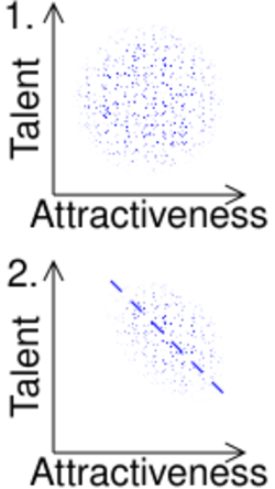
In figure 1, assume that talent and attractiveness are uncorrelated in the population.
In figure 2, someone sampling the population using celebrities may wrongly infer that talent is negatively correlated with attractiveness, as people who are neither talented nor attractive do not typically become celebrities.
Berkson's paradox, also known as Berkson's bias, collider bias, or Berkson's fallacy, is a result in conditional probability and statistics which is often found to be counterintuitive, and hence a veridical paradox. It is a complicating factor arising in statistical tests of proportions. Specifically, it arises when there is an ascertainment bias inherent in a study design. The effect is related to the explaining away phenomenon in Bayesian networks, and conditioning on a collider in graphical models.
It is often described in the fields of medical statistics or biostatistics, as in the original description of the problem by Joseph Berkson.
Examples
Overview

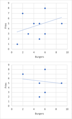
The most common example of Berkson's paradox is a false observation of a negative correlation between two desirable traits, i.e., that members of a population which have some desirable trait tend to lack a second. Berkson's paradox occurs when this observation appears true when in reality the two properties are unrelated—or even positively correlated—because members of the population where both are absent are not equally observed. For example, a person may observe from their experience that fast food restaurants in their area which serve good hamburgers tend to serve bad fries and vice versa; but because they would likely not eat anywhere where both were bad, they fail to allow for the large number of restaurants in this category which would weaken or even flip the correlation.
Original illustration
Berkson's original illustration involves a retrospective study examining a risk factor for a disease in a statistical sample from a hospital in-patient population. Because samples are taken from a hospital in-patient population, rather than from the general public, this can result in a spurious negative association between the disease and the risk factor. For example, if the risk factor is diabetes and the disease is cholecystitis, a hospital patient without diabetes is more likely to have cholecystitis than a member of the general population, since the patient must have had some non-diabetes (possibly cholecystitis-causing) reason to enter the hospital in the first place. That result will be obtained regardless of whether there is any association between diabetes and cholecystitis in the general population.
Ellenberg example
An example presented by Jordan Ellenberg: Suppose Alex will only date a man if his niceness plus his handsomeness exceeds some threshold. Then nicer men do not have to be as handsome to qualify for Alex's dating pool. So, among the men that Alex dates, Alex may observe that the nicer ones are less handsome on average (and vice versa), even if these traits are uncorrelated in the general population. Note that this does not mean that men in the dating pool compare unfavorably with men in the population. On the contrary, Alex's selection criterion means that Alex has high standards. The average nice man that Alex dates is actually more handsome than the average man in the population (since even among nice men, the ugliest portion of the population is skipped). Berkson's negative correlation is an effect that arises within the dating pool: the rude men that Alex dates must have been even more handsome to qualify.
Quantitative example
As a quantitative example, suppose a collector has 1000 postage stamps, of which 300 are pretty and 100 are rare, with 30 being both pretty and rare. 30% of all his stamps are pretty and 10% of his pretty stamps are rare, so prettiness tells nothing about rarity. He puts the 370 stamps which are pretty or rare on display. Just over 27% of the stamps on display are rare (100/370), but still only 10%(30/300) of the pretty stamps are rare (and 100% of the 70 not-pretty stamps on display are rare). If an observer only considers stamps on display, they will observe a spurious negative relationship between prettiness and rarity as a result of the selection bias (that is, not-prettiness strongly indicates rarity in the display, but not in the total collection).
Statement
Two independent events become conditionally dependent given that at least one of them occurs. Symbolically:
- If [math]\displaystyle{ 0 \lt P(A) \lt 1 }[/math], [math]\displaystyle{ 0 \lt P(B) \lt 1 }[/math], and [math]\displaystyle{ P(A|B) = P(A) }[/math], then [math]\displaystyle{ P(A|B,A \cup B) = P(A) }[/math] and hence [math]\displaystyle{ P(A|A \cup B) \gt P(A) }[/math].
- Event [math]\displaystyle{ A }[/math] and event [math]\displaystyle{ B }[/math] may or may not occur.
- [math]\displaystyle{ P(A \mid B) }[/math], a conditional probability, is the probability of observing event [math]\displaystyle{ A }[/math] given that [math]\displaystyle{ B }[/math] is true.
- Explanation: Event [math]\displaystyle{ A }[/math] and [math]\displaystyle{ B }[/math] are independent of each other.
- [math]\displaystyle{ P(A \mid B,A \cup B) }[/math] is the probability of observing event [math]\displaystyle{ A }[/math] given that [math]\displaystyle{ B }[/math] and ([math]\displaystyle{ A }[/math] or [math]\displaystyle{ B }[/math]) occurs. This can also be written as [math]\displaystyle{ P(A \mid B \cap (A \cup B)) }[/math].
- Explanation: The probability of [math]\displaystyle{ A }[/math] given both [math]\displaystyle{ B }[/math] and ([math]\displaystyle{ A }[/math] or [math]\displaystyle{ B }[/math]) is smaller than the probability of [math]\displaystyle{ A }[/math] given ([math]\displaystyle{ A }[/math] or [math]\displaystyle{ B }[/math])
In other words, given two independent events, if you consider only outcomes where at least one occurs, then they become conditionally dependent, as shown above.
There's a simpler, more general argument:
Given two events [math]\displaystyle{ A }[/math] and [math]\displaystyle{ B }[/math] with [math]\displaystyle{ 0 \lt P(A) \leq 1 }[/math], we have [math]\displaystyle{ 0 \lt P(A) \leq P(A \cup B) \leq 1 }[/math]. Multiplying both sides of the right-hand inequality by [math]\displaystyle{ P(A) }[/math], we get [math]\displaystyle{ P(A)P(A \cup B) \leq P(A) }[/math]. Dividing both sides of this by [math]\displaystyle{ P(A \cup B) }[/math] yields [math]\displaystyle{ \begin{align} P(A) \leq \frac{P(A)}{P(A \cup B)} & = \frac{P(A \cap (A \cup B))}{P(A \cup B)} \\ &= P(A \mid A \cup B), i.e., P(A) \leq P(A \mid A \cup B) \end{align} }[/math]
When [math]\displaystyle{ P(A \cup B) \lt 1 }[/math] (i.e., when [math]\displaystyle{ A \cup B }[/math] is a set of less than full probability), the inequality is strict: [math]\displaystyle{ P(A) \lt P(A \mid A \cup B) }[/math], and hence, [math]\displaystyle{ A }[/math] and [math]\displaystyle{ A \cup B }[/math] are dependent.
Note only two assumptions were used in the argument above: (i) [math]\displaystyle{ 0 \lt P(A) \leq 1 }[/math] which is sufficient to imply [math]\displaystyle{ P(A) \leq P(A \mid A \cup B) }[/math]. And (ii) [math]\displaystyle{ P(A \cup B) \lt 1 }[/math], which with (i) implies the strict inequality [math]\displaystyle{ P(A) \lt P(A \mid A \cup B) }[/math], and so dependence of [math]\displaystyle{ A }[/math] and [math]\displaystyle{ A \cup B }[/math]. It's not necessary to assume [math]\displaystyle{ A }[/math] and [math]\displaystyle{ B }[/math] are independent—it's true for any events [math]\displaystyle{ A }[/math] and [math]\displaystyle{ B }[/math] satisfying (i) and (ii) (including independent events).
Explanation
The cause is that the conditional probability of event [math]\displaystyle{ A }[/math] occurring, given that it or [math]\displaystyle{ B }[/math] occurs, is inflated: it is higher than the unconditional probability, because we have excluded cases where neither occur.
- [math]\displaystyle{ P(A \mid A \cup B) \gt P(A) }[/math]
- conditional probability inflated relative to unconditional
One can see this in tabular form as follows: the yellow regions are the outcomes where at least one event occurs (and ~A means "not A").
| A | ~A | |
|---|---|---|
| B | A & B | ~A & B |
| ~B | A & ~B | ~A & ~B |
For instance, if one has a sample of [math]\displaystyle{ 100 }[/math], and both [math]\displaystyle{ A }[/math] and [math]\displaystyle{ B }[/math] occur independently half the time ( [math]\displaystyle{ P(A) = P(B) = 1 / 2 }[/math] ), one obtains:
| A | ~A | |
|---|---|---|
| B | 25 | 25 |
| ~B | 25 | 25 |
So in [math]\displaystyle{ 75 }[/math] outcomes, either [math]\displaystyle{ A }[/math] or [math]\displaystyle{ B }[/math] occurs, of which [math]\displaystyle{ 50 }[/math] have [math]\displaystyle{ A }[/math] occurring. By comparing the conditional probability of [math]\displaystyle{ A }[/math] to the unconditional probability of [math]\displaystyle{ A }[/math]:
- [math]\displaystyle{ P(A|A \cup B) = 50 / 75 = 2 / 3 \gt P(A) = 50 / 100 = 1 / 2 }[/math]
We see that the probability of [math]\displaystyle{ A }[/math] is higher ([math]\displaystyle{ 2 / 3 }[/math]) in the subset of outcomes where ([math]\displaystyle{ A }[/math] or [math]\displaystyle{ B }[/math]) occurs, than in the overall population ([math]\displaystyle{ 1 / 2 }[/math]). On the other hand, the probability of [math]\displaystyle{ A }[/math] given both [math]\displaystyle{ B }[/math] and ([math]\displaystyle{ A }[/math] or [math]\displaystyle{ B }[/math]) is simply the unconditional probability of [math]\displaystyle{ A }[/math], [math]\displaystyle{ P(A) }[/math], since [math]\displaystyle{ A }[/math] is independent of [math]\displaystyle{ B }[/math]. In the numerical example, we have conditioned on being in the top row:
| A | ~A | |
|---|---|---|
| B | 25 | 25 |
| ~B | 25 | 25 |
Here the probability of [math]\displaystyle{ A }[/math] is [math]\displaystyle{ 25 / 50 = 1 / 2 }[/math].
Berkson's paradox arises because the conditional probability of [math]\displaystyle{ A }[/math] given [math]\displaystyle{ B }[/math] within the three-cell subset equals the conditional probability in the overall population, but the unconditional probability within the subset is inflated relative to the unconditional probability in the overall population, hence, within the subset, the presence of [math]\displaystyle{ B }[/math] decreases the conditional probability of [math]\displaystyle{ A }[/math] (back to its overall unconditional probability):
- [math]\displaystyle{ P(A|B, A \cup B) = P(A|B) = P(A) }[/math]
- [math]\displaystyle{ P(A|A \cup B) \gt P(A) }[/math]
Because the effect of conditioning on [math]\displaystyle{ (A \cup B) }[/math] derives from the relative size of [math]\displaystyle{ P(A|A \cup B) }[/math] and [math]\displaystyle{ P(A) }[/math] the effect is particularly large when [math]\displaystyle{ A }[/math] is rare ([math]\displaystyle{ P(A)\lt \lt 1 }[/math]) but very strongly correlated to [math]\displaystyle{ B }[/math] ([math]\displaystyle{ P(A|B) \approx 1 }[/math]). For example, consider the case below where N is very large:
| A | ~A | |
|---|---|---|
| B | 1 | 0 |
| ~B | 0 | N |
For the case without conditioning on [math]\displaystyle{ (A \cup B) }[/math] we have
- [math]\displaystyle{ P(A) = 1/(N+1) }[/math]
- [math]\displaystyle{ P(A|B) = 1 }[/math]
So A occurs rarely, unless B is present, when A occurs always. Thus B is dramatically increasing the likelihood of A.
For the case with conditioning on [math]\displaystyle{ (A \cup B) }[/math] we have
- [math]\displaystyle{ P(A|A \cup B) = 1 }[/math]
- [math]\displaystyle{ P(A|B, A \cup B) = P(A|B) = 1 }[/math]
Now A occurs always, whether B is present or not. So B has no impact on the likelihood of A. Thus we see that for highly correlated data a huge positive correlation of B on A can be effectively removed when one conditions on [math]\displaystyle{ (A \cup B) }[/math].
See also
References
- Berkson, Joseph (June 1946). "Limitations of the Application of Fourfold Table Analysis to Hospital Data". Biometrics Bulletin 2 (3): 47–53. doi:10.2307/3002000. PMID 21001024. (The paper is frequently miscited as Berkson, J. (1949) Biological Bulletin 2, 47–53.)
- Jordan Ellenberg, "Why are handsome men such jerks?"
 |

