Crack growth equation

A crack growth equation is used for calculating the size of a fatigue crack growing from cyclic loads. The growth of a fatigue crack can result in catastrophic failure, particularly in the case of aircraft. When many growing fatigue cracks interact with one another it is known as widespread fatigue damage. A crack growth equation can be used to ensure safety, both in the design phase and during operation, by predicting the size of cracks. In critical structure, loads can be recorded and used to predict the size of cracks to ensure maintenance or retirement occurs prior to any of the cracks failing. Safety factors are used to reduce the predicted fatigue life to a service fatigue life because of the sensitivity of the fatigue life to the size and shape of crack initiating defects and the variability between assumed loading and actual loading experienced by a component.
Fatigue life can be divided into an initiation period and a crack growth period.[1] Crack growth equations are used to predict the crack size starting from a given initial flaw and are typically based on experimental data obtained from constant amplitude fatigue tests.
One of the earliest crack growth equations based on the stress intensity factor range of a load cycle () is the Paris–Erdogan equation[2]
where is the crack length and is the fatigue crack growth for a single load cycle . A variety of crack growth equations similar to the Paris–Erdogan equation have been developed to include factors that affect the crack growth rate such as stress ratio, overloads and load history effects.
The stress intensity range can be calculated from the maximum and minimum stress intensity for a cycle
A geometry factor is used to relate the far field stress to the crack tip stress intensity using
- .
There are standard references containing the geometry factors for many different configurations.[3][4][5]
History of crack propagation equations
Many crack propagation equations have been proposed over the years to improve prediction accuracy and incorporate a variety of effects. The works of Head,[6] Frost and Dugdale,[7] McEvily and Illg,[8] and Liu[9] on fatigue crack-growth behaviour laid the foundation in this topic. The general form of these crack propagation equations may be expressed as
where, the crack length is denoted by , the number of cycles of load applied is given by , the stress range by , and the material parameters by . For symmetrical configurations, the length of the crack from the line of symmetry is defined as and is half of the total crack length .
Crack growth equations of the form are not a true differential equation as they do not model the process of crack growth in a continuous manner throughout the loading cycle. As such, separate cycle counting or identification algorithms such as the commonly used rainflow-counting algorithm, are required to identify the maximum and minimum values in a cycle. Although developed for the stress/strain-life methods rainflow counting has also been shown to work for crack growth.[10] There have been a small number of true derivative fatigue crack growth equations that have also been developed.[11][12]
Factors affecting crack growth rate
Regimes
Figure 1 shows a typical plot of the rate of crack growth as a function of the alternating stress intensity or crack tip driving force plotted on log scales. The crack growth rate behaviour with respect to the alternating stress intensity can be explained in different regimes (see, figure 1) as follows
Regime A: At low growth rates, variations in microstructure, mean stress (or load ratio), and environment have significant effects on the crack propagation rates. It is observed at low load ratios that the growth rate is most sensitive to microstructure and in low strength materials it is most sensitive to load ratio.[13]
Regime B: At mid-range of growth rates, variations in microstructure, mean stress (or load ratio), thickness, and environment have no significant effects on the crack propagation rates.
Regime C: At high growth rates, crack propagation is highly sensitive to the variations in microstructure, mean stress (or load ratio), and thickness. Environmental effects have relatively very less influence.
Stress ratio effect
Cycles with higher stress ratio have an increased rate of crack growth.[14] This effect is often explained using the crack closure concept which describes the observation that the crack faces can remain in contact with each other at loads above zero. This reduces the effective stress intensity factor range and the fatigue crack growth rate.[15]
Sequence effects
A equation gives the rate of growth for a single cycle, but when the loading is not constant amplitude, changes in the loading can lead to temporary increases or decreases in the rate of growth. Additional equations have been developed to deal with some of these cases. The rate of growth is retarded when an overload occurs in a loading sequence. These loads generate a plastic zone that may delay the rate of growth. Two notable equations for modelling the delays occurring while the crack grows through the overload region are:[16]
- The Wheeler model (1972)
- with
where is the plastic zone corresponding to the ith cycle that occurs post the overload and is the distance between the crack and the extent of the plastic zone at the overload.
- The Willenborg model
Crack growth equations
Threshold equation
To predict the crack growth rate at the near threshold region, the following relation has been used[17]
Paris–Erdoğan equation
To predict the crack growth rate in the intermediate regime, the Paris–Erdoğan equation is used[2]
Forman equation
In 1967, Forman proposed the following relation to account for the increased growth rates due to stress ratio and when approaching the fracture toughness [18]
McEvily–Groeger equation
McEvily and Groeger[19] proposed the following power-law relationship which considers the effects of both high and low values of
- .
NASGRO equation
The NASGRO equation is used in the crack growth programs AFGROW, FASTRAN and NASGRO software.[20] It is a general equation that covers the lower growth rate near the threshold and the increased growth rate approaching the fracture toughness , as well as allowing for the mean stress effect by including the stress ratio . The NASGRO equation is
where , , , , , and are the equation coefficients.
McClintock equation
In 1967, McClintock developed an equation for the upper limit of crack growth based on the cyclic crack tip opening displacement [21]
where is the flow stress, is the Young's modulus and is a constant typically in the range 0.1–0.5.
Walker equation
To account for the stress ratio effect, Walker suggested a modified form of the Paris–Erdogan equation[22]
where, is a material parameter which represents the influence of stress ratio on the fatigue crack growth rate. Typically, takes a value around , but can vary between . In general, it is assumed that compressive portion of the loading cycle has no effect on the crack growth by considering which gives This can be physically explained by considering that the crack closes at zero load and does not behave like a crack under compressive loads. In very ductile materials like Man-Ten steel, compressive loading does contribute to the crack growth according to .[23]
Elber equation
Elber modified the Paris–Erdogan equation to allow for crack closure with the introduction of the opening stress intensity level at which contact occurs. Below this level there is no movement at the crack tip and hence no growth. This effect has been used to explain the stress ratio effect and the increased rate of growth observed with short cracks. Elber's equation is[16]
Ductile and brittle materials equation
The general form of the fatigue-crack growth rate in ductile and brittle materials is given by[21]
where, and are material parameters. Based on different crack-advance and crack-tip shielding mechanisms in metals, ceramics, and intermetallics, it is observed that the fatigue crack growth rate in metals is significantly dependent on term, in ceramics on , and intermetallics have almost similar dependence on and terms.
Prediction of fatigue life
Computer programs
There are many computer programs that implement crack growth equations such as Nasgro,[24] AFGROW and Fastran. In addition, there are also programs that implement a probabilistic approach to crack growth that calculate the probability of failure throughout the life of a component.[25][26]
Crack growth programs grow a crack from an initial flaw size until it exceeds the fracture toughness of a material and fails. Because the fracture toughness depends on the boundary conditions, the fracture toughness may change from plane strain conditions for a semi-circular surface crack to plane stress conditions for a through crack. The fracture toughness for plane stress conditions is typically twice as large as that for plane strain. However, because of the rapid rate of growth of a crack near the end of its life, variations in fracture toughness do not significantly alter the life of a component.
Crack growth programs typically provide a choice of:
- cycle counting methods to extract cycle extremes
- geometry factors that select for the shape of the crack and the applied loading
- crack growth equation
- acceleration/retardation models
- material properties such as yield strength and fracture toughness
Analytical solution
The stress intensity factor is given by
where is the applied uniform tensile stress acting on the specimen in the direction perpendicular to the crack plane, is the crack length and is a dimensionless parameter that depends on the geometry of the specimen. The alternating stress intensity becomes
where is the range of the cyclic stress amplitude.
By assuming the initial crack size to be , the critical crack size before the specimen fails can be computed using as
The above equation in is implicit in nature and can be solved numerically if necessary.
Case I
For crack closure has negligible effect on the crack growth rate[27] and the Paris–Erdogan equation can be used to compute the fatigue life of a specimen before it reaches the critical crack size as
Crack growth model with constant value of 𝛽 and R = 0
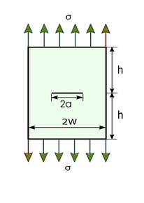
For the Griffith-Irwin crack growth model or center crack of length in an infinite sheet as shown in the figure 2, we have and is independent of the crack length. Also, can be considered to be independent of the crack length. By assuming the above integral simplifies to
by integrating the above expression for and cases, the total number of load cycles are given by
Now, for and critical crack size to be very large in comparison to the initial crack size will give
The above analytical expressions for the total number of load cycles to fracture are obtained by assuming . For the cases, where is dependent on the crack size such as the Single Edge Notch Tension (SENT), Center Cracked Tension (CCT) geometries, numerical integration can be used to compute .
Case II
For crack closure phenomenon has an effect on the crack growth rate and we can invoke Walker equation to compute the fatigue life of a specimen before it reaches the critical crack size as
Numerical calculation
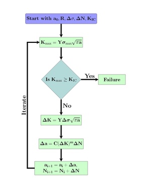
This scheme is useful when is dependent on the crack size . The initial crack size is considered to be . The stress intensity factor at the current crack size is computed using the maximum applied stress as
If is less than the fracture toughness , the crack has not reached its critical size and the simulation is continued with the current crack size to calculate the alternating stress intensity as
Now, by substituting the stress intensity factor in Paris–Erdogan equation, the increment in the crack size is computed as
where is cycle step size. The new crack size becomes
where index refers to the current iteration step. The new crack size is used to calculate the stress intensity at maximum applied stress for the next iteration. This iterative process is continued until
Once this failure criterion is met, the simulation is stopped.
The schematic representation of the fatigue life prediction process is shown in figure 3.
Example
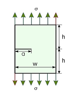
The stress intensity factor in a SENT specimen (see, figure 4) under fatigue crack growth is given by[5]
The following parameters are considered for the calculation
- mm, mm, mm, , ,
MPa,, .
The critical crack length, , can be computed when as
By solving the above equation, the critical crack length is obtained as .
Now, invoking the Paris–Erdogan equation gives
By numerical integration of the above expression, the total number of load cycles to failure is obtained as .
References
- ↑ Schijve, J. (January 1979). "Four lectures on fatigue crack growth". Engineering Fracture Mechanics 11 (1): 169–181. doi:10.1016/0013-7944(79)90039-0. ISSN 0013-7944. http://resolver.tudelft.nl/uuid:704226c6-658f-46b8-8cf4-68eeb56fb45a.
- ↑ 2.0 2.1 Paris, P. C.; Erdogan, F. (1963). "A critical analysis of crack propagation laws.". Journal of Basic Engineering 18 (4): 528–534. doi:10.1115/1.3656900..
- ↑ Murakami, Y.; Aoki, S. (1987). Stress Intensity Factors Handbook. Pergamon, Oxford.
- ↑ Rooke, D. P.; Cartwright, D. J. (1976). Compendium of Stress Intensity Factors. Her Majesty’s Stationery Office, London..
- ↑ 5.0 5.1 Tada, Hiroshi; Paris, Paul C.; Irwin, George R. (1 January 2000). The Stress Analysis of Cracks Handbook (Third ed.). Three Park Avenue New York, NY 10016-5990: ASME. doi:10.1115/1.801535. ISBN 0791801535. https://asmedigitalcollection.asme.org/ebooks/book/188/The-Stress-Analysis-of-Cracks-Handbook-Third.
- ↑ Head, A. K. (September 1953). "The growth of fatigue cracks". The London, Edinburgh, and Dublin Philosophical Magazine and Journal of Science 44 (356): 925–938. doi:10.1080/14786440908521062. ISSN 1941-5982.
- ↑ Frost, N. E.; Dugdale, D. S. (January 1958). "The propagation of fatigue cracks in sheet specimens". Journal of the Mechanics and Physics of Solids 6 (2): 92–110. doi:10.1016/0022-5096(58)90018-8. ISSN 0022-5096. Bibcode: 1958JMPSo...6...92F.
- ↑ McEvily, Arthur J.; Illg, Walter (1960). "A Method for Predicting the Rate of Fatigue-Crack Propagation". Symposium on Fatigue of Aircraft Structures. ASTM International. pp. 112–112–8. doi:10.1520/stp45927s. ISBN 9780803165793.
- ↑ Liu, H. W. (1961). "Crack Propagation in Thin Metal Sheet Under Repeated Loading". Journal of Basic Engineering 83 (1): 23–31. doi:10.1115/1.3658886. ISSN 0021-9223.
- ↑ Sunder, R.; Seetharam, S. A.; Bhaskaran, T. A. (1984). "Cycle counting for fatigue crack growth analysis". International Journal of Fatigue 6 (3): 147–156. doi:10.1016/0142-1123(84)90032-X.
- ↑ Pommier, S.; Risbet, M. (2005). "Time derivative equations for mode I fatigue crack growth in metals". International Journal of Fatigue 27 (10–12): 1297–1306. doi:10.1016/j.ijfatigue.2005.06.034.
- ↑ Lu, Zizi; Liu, Yongming (2010). "Small time scale fatigue crack growth analysis". International Journal of Fatigue 32 (8): 1306–1321. doi:10.1016/j.ijfatigue.2010.01.010.
- ↑ Ritchie, R. O. (1977). "Near-Threshold Fatigue Crack Propagation in Ultra-High Strength Steel: Influence of Load Ratio and Cyclic Strength". Journal of Engineering Materials and Technology 99 (3): 195–204. doi:10.1115/1.3443519. ISSN 0094-4289. https://escholarship.org/uc/item/3wq7226r.
- ↑ Maddox, S. J. (1975). "The effect of mean stress on fatigue crack propagation—A literature review". International Journal of Fracture 1 (3).
- ↑ Elber, W. (1971), "The Significance of Fatigue Crack Closure", Damage Tolerance in Aircraft Structures, ASTM International, pp. 230–242, doi:10.1520/stp26680s, ISBN 9780803100312
- ↑ 16.0 16.1 Suresh, S. (2004). Fatigue of Materials. Cambridge University Press. ISBN 978-0-521-57046-6.
- ↑ Allen, R. J.; Booth, G. S.; Jutla, T. (March 1988). "A review of fatigue crack growth characterisation by Linear Elastic Fracture Mechanics (LEFM). Part II – Advisory documents and applications within National Standards". Fatigue & Fracture of Engineering Materials & Structures 11 (2): 71–108. doi:10.1111/j.1460-2695.1988.tb01162.x. ISSN 8756-758X.
- ↑ Forman, R. G.; Kearney, V. E.; Engle, R. M. (1967). "Numerical Analysis of Crack Propagation in Cyclic-Loaded Structures". Journal of Basic Engineering 89 (3): 459–463. doi:10.1115/1.3609637. ISSN 0021-9223.
- ↑ McEvily, A. J.; Groeger, J. (1978), "On the threshold for fatigue crack growth", Advances in Research on the Strength and Fracture of Materials (Elsevier): pp. 1293–1298, doi:10.1016/b978-0-08-022140-3.50087-2, ISBN 9780080221403, http://www.gruppofrattura.it/ocs/index.php/ICF/ICF4/paper/view/2448
- ↑ Forman, R. G.; Shivakumar, V.; Cardinal, J. W.; Williams, L. C.; McKeighan, P.C. (2005). "Fatigue Crack Growth Database for Damage Tolerance Analysis". FAA. http://www.tc.faa.gov/its/worldpac/techrpt/ar05-15.pdf.
- ↑ 21.0 21.1 Ritchie, R. O. (1 November 1999). "Mechanisms of fatigue-crack propagation in ductile and brittle solids". International Journal of Fracture 100 (1): 55–83. doi:10.1023/A:1018655917051. ISSN 1573-2673.
- ↑ Walker, K. (1970), "The Effect of Stress Ratio During Crack Propagation and Fatigue for 2024-T3 and 7075-T6 Aluminum", Effects of Environment and Complex Load History on Fatigue Life, ASTM International, pp. 1–14, doi:10.1520/stp32032s, ISBN 9780803100329
- ↑ Dowling, Norman E. (2012). Mechanical behavior of materials: engineering methods for deformation, fracture, and fatigue. Pearson. ISBN 978-0131395060. OCLC 1055566537.
- ↑ "NASGRO® Fracture Mechanics & Fatigue Crack Growth Software". 26 September 2016. https://www.swri.org/consortia/nasgro.
- ↑ "Update of the Probability of Fracture (PROF) Computer Program for Aging Aircraft Risk Analysis. Volume 1: Modifications and User's Guide". https://www.researchgate.net/publication/235184910.
- ↑ "DARWIN Fracture mechanics and reliability assessment software". 14 October 2016. https://www.swri.org/darwin.
- ↑ Zehnder, Alan T. (2012). Fracture Mechanics. Lecture Notes in Applied and Computational Mechanics. 62. Dordrecht: Springer Netherlands. doi:10.1007/978-94-007-2595-9. ISBN 9789400725942.
- ↑ "Fatigue Crack Growth". https://mechanicalc.com/reference/fatigue-crack-growth.
External links
- Forman, R. G.; Shivakumar, V.; Cardinal, J. W.; Williams, L. C.; McKeighan, P. C. (2005). "Fatigue Crack Growth Database for Damage Tolerance Analysis". FAA. http://www.tc.faa.gov/its/worldpac/techrpt/ar05-15.pdf.
- Gallagher, J. P.; Giessler, F. J.; Berens, A. P.; Engle, Jr, J. M.. "USAF Damage Tolerant Design Handbook: Guidelines for the Analysis and Design of Damage Tolerant Aircraft Structures. Revision B". https://apps.dtic.mil/docs/citations/ADA153161.
- "Damage Tolerance Assessment Handbook Volume I: Introduction, Fracture Mechanics, Fatigue Crack Propagation". Federal Aviation Administration. 1993. http://www.tc.faa.gov/its/worldpac/techrpt/ct93-69-1.pdf.
 |  |
