EigenMoments

Signal space is transformed into moment space, i.e. Geometric Moments, then it is transformed into noise space in which axes with lowest rate of noise are retained and finally transformed into feature space

EigenMoments is a set of orthogonal, noise robust, invariant to rotation, scaling and translation and distribution sensitive moments. Their application can be found in signal processing and computer vision as descriptors of the signal or image. The descriptors can later be used for classification purposes.

It is obtained by performing orthogonalization, via eigen analysis on geometric moments.

Framework summary

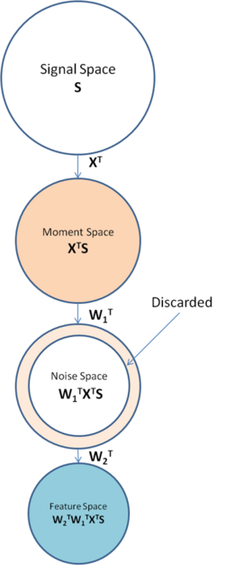
EigenMoments are computed by performing eigen analysis on the moment space of an image by maximizing signal-to-noise ratio in the feature space in form of Rayleigh quotient.

This approach has several benefits in Image processing applications:

1. Dependency of moments in the moment space on the distribution of the images being transformed, ensures decorrelation of the final feature space after eigen analysis on the moment space.
2. The ability of EigenMoments to take into account distribution of the image makes it more versatile and adaptable for different genres.
3. Generated moment kernels are orthogonal and therefore analysis on the moment space becomes easier. Transformation with orthogonal moment kernels into moment space is analogous to projection of the image onto a number of orthogonal axes.
4. Nosiy components can be removed. This makes EigenMoments robust for classification applications.
5. Optimal information compaction can be obtained and therefore a few number of moments are needed to characterize the images.

Problem formulation

Assume that a signal vector [math]\displaystyle{ s \in \mathcal{R}^n }[/math] is taken from a certain distribution having coorelation [math]\displaystyle{ C \in \mathcal{R}^{n \times n} }[/math], i.e. [math]\displaystyle{ C=E[ss^T] }[/math] where E[.] denotes expected value.

Dimension of signal space, n, is often too large to be useful for practical application such as pattern classification, we need to transform the signal space into a space with lower dimensionality.

This is performed by a two-step linear transformation:

[math]\displaystyle{ q=W^T X^T s, }[/math]

where [math]\displaystyle{ q=[q_1,...,q_n]^T \in \mathcal{R}^k }[/math] is the transformed signal, [math]\displaystyle{ X=[x_1,...,x_n]^T \in \mathcal{R}^{n \times m} }[/math] a fixed transformation matrix which transforms the signal into the moment space, and [math]\displaystyle{ W=[w_1,...,w_n]^T \in \mathcal{R}^{m \times k} }[/math] the transformation matrix which we are going to determine by maximizing the SNR of the feature space resided by [math]\displaystyle{ q }[/math]. For the case of Geometric Moments, X would be the monomials. If [math]\displaystyle{ m=k=n }[/math], a full rank transformation would result, however usually we have [math]\displaystyle{ m \leq n }[/math] and [math]\displaystyle{ k \leq m }[/math]. This is specially the case when [math]\displaystyle{ n }[/math] is of high dimensions.

Finding [math]\displaystyle{ W }[/math] that maximizes the SNR of the feature space:

[math]\displaystyle{ SNR_{transform} = \frac{w^TX^TCXw}{w^TX^TNXw}, }[/math]

where N is the correlation matrix of the noise signal. The problem can thus be formulated as

[math]\displaystyle{ {w_1,...,w_k}=argmax_w \frac{w^TX^TCXw}{w^TX^TNXw} }[/math]

subject to constraints:

[math]\displaystyle{ w_i^T X^T NX w_j=\delta_{ij}, }[/math] where [math]\displaystyle{ \delta_{ij} }[/math] is the Kronecker delta.

It can be observed that this maximization is Rayleigh quotient by letting [math]\displaystyle{ A=X^TCX }[/math] and [math]\displaystyle{ B=X^TNX }[/math] and therefore can be written as:

[math]\displaystyle{ {w_1,...,w_k}=\underset{x}{\operatorname{arg\,max}} \frac{w^TAw}{w^TBw} }[/math], [math]\displaystyle{ w_i^TBw_j=\delta_{ij} }[/math]

Rayleigh quotient

Optimization of Rayleigh quotient has the form:

[math]\displaystyle{ \max_w R(w)= \max_w \frac{w^{T}Aw}{w^{T}Bw} }[/math]

and [math]\displaystyle{ A }[/math] and [math]\displaystyle{ B }[/math], both are symmetric and [math]\displaystyle{ B }[/math] is positive definite and therefore invertible. Scaling [math]\displaystyle{ w }[/math] does not change the value of the object function and hence and additional scalar constraint [math]\displaystyle{ w^{T}Bw=1 }[/math] can be imposed on [math]\displaystyle{ w }[/math] and no solution would be lost when the objective function is optimized.

This constraint optimization problem can be solved using Lagrangian multiplier:

[math]\displaystyle{ \max_w {w^{T}Aw} }[/math] subject to [math]\displaystyle{ {w^{T}Bw}=1 }[/math]

[math]\displaystyle{ \max_w \mathcal{L}(w) = \max_w (w{T}Aw-\lambda w^{T}Bw) }[/math]

equating first derivative to zero and we will have:

[math]\displaystyle{ Aw=\lambda Bw }[/math]

which is an instance of Generalized Eigenvalue Problem (GEP). The GEP has the form:

[math]\displaystyle{ Aw=\lambda Bw }[/math]

for any pair [math]\displaystyle{ (w,\lambda) }[/math] that is a solution to above equation, [math]\displaystyle{ w }[/math] is called a generalized eigenvector and [math]\displaystyle{ \lambda }[/math] is called a generalized eigenvalue.

Finding [math]\displaystyle{ w }[/math] and [math]\displaystyle{ \lambda }[/math] that satisfies this equations would produce the result which optimizes Rayleigh quotient.

One way of maximizing Rayleigh quotient is through solving the Generalized Eigen Problem. Dimension reduction can be performed by simply choosing the first components [math]\displaystyle{ w_i }[/math], [math]\displaystyle{ i=1,...,k }[/math], with the highest values for [math]\displaystyle{ R(w) }[/math] out of the [math]\displaystyle{ m }[/math] components, and discard the rest. Interpretation of this transformation is rotating and scaling the moment space, transforming it into a feature space with maximized SNR and therefore, the first [math]\displaystyle{ k }[/math] components are the components with highest [math]\displaystyle{ k }[/math] SNR values.

The other method to look at this solution is to use the concept of simultaneous diagonalization instead of Generalized Eigen Problem.

Simultaneous diagonalization

1. Let [math]\displaystyle{ A=X^TCX }[/math] and [math]\displaystyle{ B=X^TNX }[/math] as mentioned earlier. We can write [math]\displaystyle{ W }[/math] as two separate transformation matrices:

[math]\displaystyle{ W=W_1W_2. }[/math]

1. [math]\displaystyle{ W_1 }[/math] can be found by first diagonalize B:

[math]\displaystyle{ P^TBP=D_B }[/math].

Where [math]\displaystyle{ D_B }[/math] is a diagonal matrix sorted in increasing order. Since [math]\displaystyle{ B }[/math] is positive definite, thus [math]\displaystyle{ D_B\gt 0 }[/math]. We can discard those eigenvalues that large and retain those close to 0, since this means the energy of the noise is close to 0 in this space, at this stage it is also possible to discard those eigenvectors that have large eigenvalues.

Let [math]\displaystyle{ \hat P }[/math] be the first [math]\displaystyle{ k }[/math] columns of [math]\displaystyle{ P }[/math], now [math]\displaystyle{ \hat{P^T}B\hat P=\hat{D_B} }[/math] where [math]\displaystyle{ \hat{D_B} }[/math] is the [math]\displaystyle{ k \times k }[/math] principal submatrix of [math]\displaystyle{ D_B }[/math].

1. Let

[math]\displaystyle{ W_1=\hat{P} \hat{D_B}^{-1/2} }[/math]

and hence:

[math]\displaystyle{ W_1^T B W_1=(\hat P \hat{D_B}^{-1/2})^TB(\hat P \hat{D_B}^{-1/2})=I }[/math].

[math]\displaystyle{ W_1 }[/math] whiten [math]\displaystyle{ B }[/math] and reduces the dimensionality from [math]\displaystyle{ m }[/math] to [math]\displaystyle{ k }[/math]. The transformed space resided by [math]\displaystyle{ q'=W_1^TX^Ts }[/math] is called the noise space.

1. Then, we diagonalize [math]\displaystyle{ W_1^T A W_1 }[/math]:

[math]\displaystyle{ W_2^T W_1^T A W_1 W_2 = D_A }[/math],

where [math]\displaystyle{ W_2^T W_2 =I }[/math]. [math]\displaystyle{ D_A }[/math] is the matrix with eigenvalues of [math]\displaystyle{ W_1^T A W_1 }[/math] on its diagonal. We may retain all the eigenvalues and their corresponding eigenvectors since the most of the noise are already discarded in previous step.

1. Finally the transformation is given by:

[math]\displaystyle{ W=W_1W_2 }[/math]

where [math]\displaystyle{ W }[/math] diagonalizes both the numerator and denominator of the SNR,

[math]\displaystyle{ W^TAW=D_A }[/math], [math]\displaystyle{ W^TBW=I }[/math] and the transformation of signal [math]\displaystyle{ s }[/math] is defined as [math]\displaystyle{ q=W^TX^Ts=W_2^TW_1^TX^Ts }[/math].

Information loss

To find the information loss when we discard some of the eigenvalues and eigenvectors we can perform following analysis:

[math]\displaystyle{ \begin{array}{lll} \eta &=& 1- \frac{trace(W_1^TAW_1)}{trace(D_B^{-1/2}P^TAPD_B^{-1/2})}\\ &=& 1- \frac{trace(\hat{D_B}^{-1/2}\hat{P}^TA\hat{P}\hat{D_B}^{-1/2})}{trace(D_B^{-1/2}P^TAPD_B^{-1/2})} \end{array} }[/math]

Eigenmoments

Eigenmoments are derived by applying the above framework on Geometric Moments. They can be derived for both 1D and 2D signals.

1D signal

If we let [math]\displaystyle{ X=[1,x,x^2,...,x^{m-1}] }[/math], i.e. the monomials, after the transformation [math]\displaystyle{ X^T }[/math] we obtain Geometric Moments, denoted by vector [math]\displaystyle{ M }[/math], of signal [math]\displaystyle{ s=[s(x)] }[/math],i.e. [math]\displaystyle{ M=X^Ts }[/math].

In practice it is difficult to estimate the correlation signal due to insufficient number of samples, therefore parametric approaches are utilized.

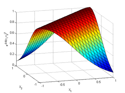
One such model can be defined as:

[math]\displaystyle{ r(x_1,x_2)=r(0,0)e^{-c(x_1-x_2)^2} }[/math],

Plot of the parametric model which predicts correlations in the input signal. [math]\displaystyle{ r(x_1,x_2)=r(0,0)e^{-c(x_1-x_2)^2} }[/math]

where [math]\displaystyle{ r(0,0)=E[tr(ss^T)] }[/math]. This model of correlation can be replaced by other models however this model covers general natural images.

Since [math]\displaystyle{ r(0,0) }[/math] does not affect the maximization it can be dropped.

[math]\displaystyle{ A=X^TCX=\int_{-1}^{1}\int_{-1}^{1}[x_1^j x_2^i e^{-c(x_1-x_2)^2}]_{i,j=0}^{i,j=m-1}dx_1dx_2 }[/math]

The correlation of noise can be modelled as [math]\displaystyle{ \sigma_n^2\delta(x_1,x_2) }[/math], where [math]\displaystyle{ \sigma_n^2 }[/math] is the energy of noise. Again [math]\displaystyle{ \sigma_n^2 }[/math] can be dropped because the constant does not have any effect on the maximization problem.

[math]\displaystyle{ B=X^TNX=\int_{-1}^{1}\int_{-1}^{1}[x_1^j x_2^i\delta(x_1,x_2)]_{i,j=0}^{i,j=m-1}dx_1dx_2 }[/math] [math]\displaystyle{ B=X^TNX=\int_{-1}^{1}[x_1^{j+i}]_{i,j=0}^{i,j=m-1}dx_1=X^TX }[/math]

Using the computed A and B and applying the algorithm discussed in previous section we find [math]\displaystyle{ W }[/math] and set of transformed monomials [math]\displaystyle{ \Phi=[\phi_1,...,\phi_k]=XW }[/math] which produces the moment kernels of EM. The moment kernels of EM decorrelate the correlation in the image.

[math]\displaystyle{ \Phi^TC\Phi=(XW)^TC(XW)=D_C }[/math],

and are orthogonal:

[math]\displaystyle{ \begin{array}{lll}\Phi^T\Phi& = & (XW)^T(XW) \\ & = & W^TX^TX\\ & = & W^TX^TNXW\\ & = & W^TBW\\ & = & I\\ \end{array} }[/math]

Example computation

Taking [math]\displaystyle{ c=0.5 }[/math], the dimension of moment space as [math]\displaystyle{ m=6 }[/math] and the dimension of feature space as [math]\displaystyle{ k=4 }[/math], we will have:

[math]\displaystyle{ W= \left( \begin{array}{cccc} 0.0 & 0 & -0.7745 & -0.8960 \\ 2.8669 & -4.4622 & 0.0 & 0.0 \\ 0.0 & 0.0 & 7.9272 & 2.4523 \\ -4.0225 & 20.6505 & 0.0 & 0.0 \\ 0.0 & 0.0 & -9.2789 & -0.1239 \\ -0.5092 & -18.4582 & 0.0 & 0.0 \end{array} \right) }[/math]

and

[math]\displaystyle{ \begin{array}{lll} \phi_1&=& 2.8669x - 4.0225x^3 - 0.5092x^5 \\ \phi_2&=&-4.4622x + 20.6505x^3 - 18.4582x^5 \\ \phi_3&=&-0.7745 + 7.9272x^2 - 9.2789x^4 \\ \phi_4&=&-0.8960 + 2.4523x^2 - 0.1239x^4 \\ \end{array} }[/math]

2D signal

The derivation for 2D signal is the same as 1D signal except that conventional Geometric Moments are directly employed to obtain the set of 2D EigenMoments.

The definition of Geometric Moments of order [math]\displaystyle{ (p+q) }[/math] for 2D image signal is:

[math]\displaystyle{ m_{pq}=\int_{-1}^1\int_{-1}^1 x^py^qf(x,y)dxdy }[/math].

which can be denoted as [math]\displaystyle{ M=\{m_{j,i}\}_{i,j=0}^{i,j=m-1} }[/math]. Then the set of 2D EigenMoments are:

[math]\displaystyle{ \Omega=W^TMW }[/math],

where [math]\displaystyle{ \Omega=\{\Omega_{j,i}\}_{i,j=0}^{i,j=k-1} }[/math] is a matrix that contains the set of EigenMoments.

[math]\displaystyle{ \Omega_{j,i}=\Sigma_{r=0}^{m-1}\Sigma_{s=0}^{m-1}w_{r,j}w_{s,i}m_{r,s} }[/math].

EigenMoment invariants (EMI)

In order to obtain a set of moment invariants we can use normalized Geometric Moments [math]\displaystyle{ \hat M }[/math] instead of [math]\displaystyle{ M }[/math].

Normalized Geometric Moments are invariant to Rotation, Scaling and Transformation and defined by:

[math]\displaystyle{ \begin{array}{lll} \hat m_{pq} & = & \alpha^p+q+2\int_{-1}^{1}\int_{-1}^{1}[(x-x^c)cos(\theta)+(y-y^c)sin(\theta)]^p\\ & = & \times [-(x-x^c)sin(\theta)+(y-y^c)cos(\theta)]^q\\ & = & \times f(x,y)dxdy,\\ \end{array} }[/math]

where:[math]\displaystyle{ (x^c,y^c) = (m_{10}/m_{00},m_{01}/m_{00}) }[/math] is the centroid of the image [math]\displaystyle{ f(x,y) }[/math] and

[math]\displaystyle{ \begin{array}{lll} \alpha&=&[m_{00}^{S}/m_{00}]^{1/2}\\ \theta&=&\frac{1}{2}tan^{-1}\frac{2m_{11}}{m_{20}-m_{02}} \end{array} }[/math].

[math]\displaystyle{ m_{00}^{S} }[/math] in this equation is a scaling factor depending on the image. [math]\displaystyle{ m_{00}^{S} }[/math] is usually set to 1 for binary images.

See also

• Computer vision
• Signal processing
• Image moment

External links

• implementation of EigenMoments in Matlab

References

- ↑ Pew-Thian Yap, Raveendran Paramesran, Eigenmoments, Pattern Recognition, Volume 40, Issue 4, April 2007, Pages 1234-1244, ISSN 0031-3203, 10.1016/j.patcog.2006.07.003.
- ↑ M. K. Hu, "Visual Pattern Recognition by Moment Invariants", IRE Trans. Info. Theory, vol. IT-8, pp.179–187, 1962
- ↑ T. De Bie, N. Cristianini, R. Rosipal, Eigenproblems in pattern recognition, in: E. Bayro-Corrochano (Ed.), Handbook of Computational Geometry for Pattern Recognition, Computer Vision, Neurocomputing and Robotics, Springer, Heidelberg, 2004G.
- ↑ Strang, Linear Algebra and Its Applications, second ed., Academic Press, New York, 1980.