Engineering:Frequency offsets least mean squares
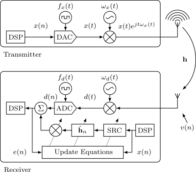
The frequency offsets least mean squares (FO-LMS) algorithm is an adaptive filter that allows estimating and tracking the channel between a transmitter and a receiver under carrier and sampling frequency offsets.[1] Frequency offsets degrade the performance of classical adaptive filters, making them unsuitable in certain cases.[2] Therefore, FO-LMS was developed to explicitly estimate the channel as well as the carrier and sampling frequency offsets. Like the classical least mean squares (LMS) adaptive filter, FO-LMS is a stochastic gradient descent method, which means that the algorithm's decisions made at each and every iteration are based on the instantaneous estimate of the actual gradient. This makes the FO-LMS a robust algorithm with low computational burder, albeit with slow convergence rate. The ability to estimate and track carrier and sampling frequency offsets in addition to the channel makes FO-LMS suitable for applications where the transmitted signal or parts of it are known but where frequency offsets are detrimental to performance, such as bistatic radars, orthogonal frequency-division multiplexing communication systems, or interference cancellation.[3]
Algorithm description
The FO-LMS algorithm is applicable when a transmitted signal [math]\displaystyle{ x(t) }[/math], which in its discrete-time baseband complex form [math]\displaystyle{ x(n) }[/math] is known to the receiver, is received due to the channel and frequency offsets as
- [math]\displaystyle{ d(n) = \mathbf{h}^{H} \mathbf{y}_n e^{j\sum^n_{i=1}{\epsilon(i)}} + v(n) }[/math],
where [math]\displaystyle{ v(n) }[/math] is the measurement noise, [math]\displaystyle{ \mathbf{h} }[/math] denotes the finite complex-valued impulse response of the channel with length [math]\displaystyle{ M }[/math], the multiplicative term [math]\displaystyle{ e^{j\sum^n_{i=1}{\epsilon(i)}} }[/math] accounts for the carrier frequency offset, and [math]\displaystyle{ \mathbf{y}_n }[/math] accounts for sampling [math]\displaystyle{ x(t) }[/math] with sampling frequency offset [math]\displaystyle{ \eta(n) }[/math] so that
- [math]\displaystyle{ \mathbf{y}_n = \Bigg[x\left( \sum^{n-M+1}_{i=1}{\left(1 + \eta(i)\right)} \right), \dots, x\left( \sum^{n}_{i=1}{\left(1 + \eta(i)\right)} \right)\Bigg] }[/math].
The idea behind FO-LMS is to use the gradient descent method to find a channel estimate [math]\displaystyle{ \hat{\mathbf{h}} }[/math], carrier frequency offset estimate [math]\displaystyle{ \hat{\epsilon} }[/math], and sampling frequency offset estimate [math]\displaystyle{ \hat{\eta} }[/math] that minimize the cost function [math]\displaystyle{ C(n) = E\left\{|e(n)|^{2}\right\} }[/math], where [math]\displaystyle{ E\{\cdot\} }[/math] denotes the expected value and the estimation error at the current sample [math]\displaystyle{ n }[/math] is the difference between the received signal and the estimate of the received signal
- [math]\displaystyle{ e(n) = d(n) - \hat{\mathbf{h}}^H_{n-1} \hat{\mathbf{y}}_n e^{j \sum^n_{i=1}{\hat{\epsilon}(i-1)}} }[/math],
where [math]\displaystyle{ \hat{\mathbf{y}}_n }[/math] is the result of resampling [math]\displaystyle{ x(n) }[/math] with sampling frequency offset [math]\displaystyle{ \hat{\eta}(n) }[/math]. In practice, use of the expected value is not feasible and the algorithm relies instead on a single realization of the estimation error as is characteristic to the stochastic gradient descent method. At each and every iteration, FO-LMS updates the parameter estimates by minimizing the error so that
- [math]\displaystyle{ \hat{\mathbf{h}}_{n} = \hat{\mathbf{h}}_{n-1} + \mu_{\mathrm{h}} \hat{\mathbf{y}}_n e^{j \phi(n) } e^{*}(n) }[/math],
- [math]\displaystyle{ \hat{\epsilon}(n) = \hat{\mathrm{\epsilon}}(n-1) + \mu_{{\epsilon}} \Im{\left\{ \hat{\mathbf{h}}^H_{n-1} \hat{\mathbf{y}}_n e^{j \phi(n) } e^{*}(n) \right\}} }[/math],
- [math]\displaystyle{ \hat{\eta}(n) = \hat{\eta}(n-1) + \mu_{{\eta}} \Re{\left\{ \hat{\mathbf{h}}^H_{n-1} \hat{\mathbf{y}}'_n e^{j \phi(n) }e^{*}(n) \right\}} }[/math],
where [math]\displaystyle{ \hat{\mathbf{y}}'_n }[/math] is the derivative of [math]\displaystyle{ \hat{\mathbf{y}}_n }[/math] and can typically be calculated using first-order divided difference, [math]\displaystyle{ \phi(n) = \sum^n_{i=1} \hat{\epsilon}(i-1) }[/math] is the instantaneous phase shift caused by the estimated carrier frequency offset [math]\displaystyle{ \hat{\epsilon}(n) }[/math], [math]\displaystyle{ \Im{\{\cdot\}} }[/math] denotes the imaginary part of a complex number, [math]\displaystyle{ \Re{\{\cdot\}} }[/math] the real part, and [math]\displaystyle{ \mu_\mathrm{h} }[/math], [math]\displaystyle{ \mu_\mathrm{\epsilon} }[/math], and [math]\displaystyle{ \mu_\mathrm{\eta} }[/math] are the algorithm step sizes for controlling how rapidly the parameter estimates are advanced. Larger step sizes result in quicker convergence but also in larger excess mean squared error while in steady state.
Convergence and stability
The step sizes [math]\displaystyle{ \mu_\mathrm{h} }[/math], [math]\displaystyle{ \mu_\mathrm{\epsilon} }[/math], and [math]\displaystyle{ \mu_\mathrm{\eta} }[/math] control how quickly the algorithm converges to around-optimal parameter estimates. The algorithm never converges to the optimal parameters exactly but with suitable step sizes the parameter estimates approach and change around the optimal values. This is because the algorithm relies on a single realization of the estimation error at each iteration, rather than on the expectation. As such, the step sizes also control how close to the optimal parameters the estimates will be on average once they have approached the optimal values. Larger step sizes will cause the algorithm to magnify the estimation inaccuracies that results from using a single realization of the estimation error and the parameter estimates will vary further away from the optimal values, potentially even overshooting irrevocably and causing divergence. Useful step sizes bounds to prevent divergence are
- [math]\displaystyle{ 0 \lt \mu_w \leq \frac{2 - \mu_\epsilon | {\mathbf{y}}_n {\mathbf{w}}_{n-1}|^2 - \mu_\eta | \mathbf{y}'_n \mathbf{w}_{n-1} |^2}{\lVert {\mathbf{y}}_n\rVert^2} }[/math],
- [math]\displaystyle{ 0 \lt \mu_\epsilon \leq \frac{2 - \mu_w \lVert {\mathbf{y}}_n\rVert^2 - \mu_\eta | \mathbf{y}'_n \mathbf{w}_{n-1} |^2}{| {\mathbf{y}}_n {\mathbf{w}}_{n-1}|^2} }[/math],
- [math]\displaystyle{ 0 \lt \mu_\eta \leq \frac{2 - \mu_w \lVert {\mathbf{y}}_n\rVert^2 - \mu_\epsilon | {\mathbf{y}}_n {\mathbf{w}}_{n-1}|^2}{| \mathbf{y}'_n \mathbf{w}_{n-1} |^2} }[/math].
Inescapably the upper bound for any of the step sizes depends on the other two step sizes and, therefore, the step sizes need to be selected collectively.
See also
References
- ↑ Pärlin, K.; Riihonen, T.; Le Nir, V.; Adrat, M. (2023). "Estimating and Tracking Wireless Channels Under Carrier and Sampling Frequency Offsets". IEEE Transactions on Signal Processing 71: 1053–1066. doi:10.1109/TSP.2023.3259140. Bibcode: 2023ITSP...71.1053P.
- ↑ Yousef, N. R.; Sayed, A. H. (2002). "Ability of adaptive filters to track carrier offsets and channel nonstationarities". IEEE Transactions on Signal Processing 50 (7): 1053–1066. doi:10.1109/TSP.2002.1011194. Bibcode: 2002ITSP...50.1533Y.
- ↑ Pärlin, K.; Riihonen, T.; Turunen, M.; Le Nir, V.; Adrat, M. (2023). "Known-Interference Cancellation in Cooperative Jamming: Experimental Evaluation and Benchmark Algorithm Performance". IEEE Wireless Communications Letters 12 (9): 1598–1602. doi:10.1109/LWC.2023.3284006.
External links
- An open-source implementation of the FO-LMS algorithm is available for GNU Radio in gr-adapt (main source file).
 |


