The Fokas method, or unified transform, is an algorithmic procedure for analysing boundary value problems for linear partial differential equations and for an important class of nonlinear PDEs belonging to the so-called integrable systems. It is named after Greek mathematician Athanassios S. Fokas.
Traditionally, linear boundary value problems are analysed using either integral transforms and infinite series, or by employing appropriate fundamental solutions.
and given, can be solved via the sine-transform. The analogous problem on a finite interval can be solved via an infinite series. However, the solutions obtained via integral transforms and infinite series have several disadvantages:
1. The relevant representations are not uniformly convergent at the boundaries. For example, using the sine-transform, equations Eq.1 and Eq.2 imply
inside the integral of the rhs of Eq.3 and this would yield zero instead of
.
2. The above representations are unsuitable for numerical computations. This fact is a direct consequence of 1.
3. There exist traditional integral transforms and infinite series representations only for a very limited class of boundary value problems. For example, there does not exist the analogue of the sine-transform for solving the following simple problem:
supplemented with the initial and boundary conditions Eq.2.
For evolution PDEs, the Fokas method:
Constructs representations which are always uniformly convergent at the boundaries.
These representations can be used in a straightforward way, for example using MATLAB, for the numerical evaluation of the solution.
Constructs representations for evolution PDEs with spatial derivatives of any order.
In addition, the Fokas method constructs representations which are always of the form of the Ehrenpreis fundamental principle.
Fundamental solutions
For example, the solutions of the Laplace, modified Helmholtz and Helmholtz equations in the interior of the two-dimensional domain , can be expressed as integrals along the boundary of . However, these representations involve both the Dirichlet and the Neumann boundary values, thus since only one of these boundary values is known from the given data, the above representations are not effective. In order to obtain an effective representation, one needs to characterize the generalized Dirichlet to Neumann map; for example, for the Dirichlet problem one needs to obtain the Neumann boundary value in terms of the given Dirichlet datum.
Provides an elegant formulation of the generalised Dirichlet to Neumann map by deriving an algebraic relation, called the global relation, which couples appropriate transforms of all boundary values.
For simple domains and a variety of boundary conditions the global relation can be solved analytically. Furthermore, for the case that is an arbitrary convex polygon, the global relation can be solved numerically in a straightforward way, for example using MATLAB. Also, for the case that is a convex polygon, the Fokas method constructs an integral representation in the Fourier complex plane. By using this representation together with the global relation it is possible to compute the solution numerically inside the polygon in a straightforward semi-analytic manner.
This step is similar with the first step used for the traditional transforms. However, equation Eq.7 involves the t-transforms of both
and
, whereas in the case of the sine-transform
does not appear in the analogous equation (similarly, in the case of the cosine-transform only
appears). On the other hand, equation Eq.7 is valid in the lower-half complex
-plane, wheres the analogous equations for the sine and cosine transforms are valid only for
real. The Fokas method is based on the fact that equation Eq.7 has a large domain of validity.
2. By using the inverse Fourier transform, the global relation yields an integral representation on the real line. By deforming the real axis to a contour in the upper half -complex plane, it is possible to rewrite this expression as an integral along the contour , where is the boundary of the domain , which is the part of in the upper half complex plane, with defined by
where is defined by the requirement that solves the given PDE.Figure 1: The curve For equation Eq.5, equations Eq.6 and Eq.7 imply
In this case, , where . Thus, implies , i.e., and . The fact that the real axis can be deformed to is a consequence of the fact that the relevant integral is an analytic function of which decays in as .[1]
3. By using the global relation and by employing the transformations in the complex- plane which leave invariant, it is possible to eliminate from the integral representation of the transforms of the unknown boundary values. For equation Eq.5, , thus the relevant transformation is . Using this transformation, equation Eq.7 becomes
yields a zero contribution. Equation Eq.11 can be rewritten in a form which is consistent with the Ehrenpreis fundamental principle: if the boundary condition is specified for
, where
is a given positive constant, then using Cauchy's integral theorem, it follows that Eq.11 is equivalent with the following equation:
Uniform convergence
The unified transform constructs representations which are always uniformly convergent at the boundaries. For example, evaluating Eq.12 at , and then letting in the first term of the second integral in the rhs of Eq.12, it follows that
The change of variables , , implies that .
Numerical evaluation
It is straightforward to compute the solution numerically using quadrature after the contour has been deformed to ensure exponential decay of the integrand.[2] For simplicity we concentrate on the case that the relevant transforms can be computed analytically. For example,
For on , the term decays exponentially as . Also by deforming to where is a contour between the real axis and , it follows that for on the term also decays exponentially as . Thus, equation Eq.13 becomes
and the rhs of the above equation can be computed using MATLAB.
For the details of effective numerical quadrature using the unified transform, we refer the reader to,[2] which solves the advection-dispersion equation on the half-line. There it was found that the solution lends itself to quadrature (Gauss-Laguerre quadrature for exponential decay of integrand or Gauss–Hermite quadrature for squared exponential decay of integrand) with exponential convergence.
An Evolution Equation with Spatial Derivatives of Arbitrary order.
Suppose that is a solution of the given PDE. Then, is the boundary of the domain defined earlier.
If the given PDE contain spatial derivatives of order , then for even, the global relation involves unknowns, whereas for odd it involves or unknowns (depending on the coefficient of the highest derivative). However, using an appropriate number of transformations in the complex -plane which leave invariant, it is possible to obtain the needed number of equations, so that the transforms of the unknown boundary values can be obtained in terms of and of the given boundary data in terms of the solution of a system of algebraic equations.
A Numerical Collocation Method
The Fokas method gives rise to a novel spectral collocation method occurring in Fourier space. Recent work has extended the method and demonstrated a number of its advantages; it avoids the computation of singular integrals encountered in more traditional boundary based approaches, it is fast and easy to code up, it can be used for separable PDEs where no Green's function is known analytically and it can be made to converge exponentially with the correct choice of basis functions.
Basic method in a convex bounded polygon
Suppose that and both satisfy Laplace's equation in the interior of a convex bounded polygon . It follows that
In order to express the integrand of the above equation in terms of just the Dirichlet and Neumann boundary values, we parameterize and in terms of the arc length, , of . This leads to
In order to further simplify the global relation, we introduce the complex variable , and its conjugate . We then choose the test function , leading to the global relation for Laplace's equation:
A similar argument can also be used in the presence of a forcing term (giving a non-zero right-hand side). An identical argument works for the Helmholtz equation
and the modified Helmholtz equation
Choosing respective test functions and lead to respective global relations
and
These three cases deal with more general second order elliptic constant coefficient PDEs through a suitable linear change of variables.
The Dirichlet to Neumann map for a convex polygon
Suppose that is the interior of a bounded convex polygon specified by the corners . In this case, the global relation Eq.16 takes the form
The global relation involves unknown constants (for the Dirichlet problem, these constants are ). By evaluating the global relation at a sufficiently large number of different values of , the unknown constants can be obtained via the solution of a system of algebraic equations.
It is convenient to choose the above values of on the rays For this choice, as , the relevant system is diagonally dominant, thus its condition number is very small.[3]
Dealing with non-convexity
Whilst the global relation is valid for non-convex domains , the above collocation method becomes numerically unstable.[4] A heuristic explanation for this ill-conditioning in the case of the Laplace equation is as follows. The `test functions' grow/decay exponentially in certain directions of . When using a sufficiently large selection of complex -values, located in all directions from the origin, each side of a convex polygon will for many of these -values encounter larger test functions than do the remaining sides. This is exactly the same argument that motivates the `ray' choice of collocation points given by , which yield a diagonally dominant system. In contrast, for a non-convex polygon, boundary regions in indented regions will always be dominated by effects from other boundary parts, no matter the -value. This can easily be overcome by splitting up the domain into numerous convex regions (introducing fictitious boundaries) and matching the solution and normal derivative across these internal boundaries. Such splitting also allows the extension of the method to exterior/unbounded domains (see below).
Evaluating in the domain interior
Let be the associated fundamental solution of the PDE satisfied by . In the case of straight edges, Green's representation theorem leads to
Due to the orthogonality of the Legendre polynomials, for a given , the integrals in the above representation are Legendre expansion coefficients of certain analytic functions (written in terms of ). Hence the integrals can be computed rapidly (all at once) by expanding the functions in a Chebyshev basis (using the FFT) and then converting to a Legendre basis.[5] This can also be used to approximate the `smooth' part of the solution after adding global singular functions to take care of corner singularities.
Extension to curved boundaries and separable PDEs
The method can be extended to variable coefficient PDEs and curved boundaries in the following manner (see [6]). Suppose that is a matrix valued function, a vector valued function and a function (all sufficiently smooth) defined over . Consider the formal PDE in divergence form:
Assume that the domain is a bounded connected Lipschitz domain whose boundary consists of a finite number of vertices connected by arcs. Denote the corners of in anticlockwise order as with the side , joining to . can be parametrised by
Define along the curve and assume that . Suppose that we have a one-parameter family of solutions of the adjoint equation, , for some , where denotes the collocation set. Denoting the solution alongside by , the unit outward normal by and analogously the oblique derivative by , we define the following important transform:
For separable PDEs, a suitable one-parameter family of solutions can be constructed. If we expand each and its derivative along the boundary in Legendre polynomials, then we cover a similar approximate global relation as before. To compute the integrals that form the approximate global relation, we can use the same trick as before - expanding the function integrated against Legendre polynomials in a Chebyshev series and then converting to a Legendre series. A major advantage of the method in this scenario is that it is a boundary-based method which does not need any knowledge of the corresponding Green's function. Hence, it is more applicable than boundary integral methods in the setting of variable coefficients.
Singular functions and an exterior scattering problems
A major advantage of the above collocation method is that the basis choice (Legendre polynomials in the above discussion) can be flexibly chosen to capture local properties of the solution along each boundary. This is useful when the solution has different scalings in different regions of , but is particularly useful for capturing singular behavior, for example, near sharp corners of .
We consider the acoustic scattering problem solved in [7] by the method. The solution satisfies Helmholtz equation in with frequency , along with the Sommerfeld radiation condition at infinity:
with and where denotes the jump in across the plate. The complex collocation points are allowed precisely because of the radiation condition. To capture the endpoint singularities, we expand for in terms of weighted Chebyshev polynomials of the second kind:
where denotes the Bessel function of the first kind of order . For the derivative along , a suitable basis choice are Bessel functions of fractional order (to capture the singularity and algebraic decay at infinity).
We introduce the dimensionless frequency , where is the length of the plate. The figure below shows the convergence of the method for various . Here is the number of basis functions used to approximate the jump across the plate. The maximum relative absolute error is the maximum error of the computed solution divided by the maximum absolute value of the solution. The figure is for and shows the quadratic-exponential convergence of the method, namely the error decreases like for some positive . More complicated geometries (including different angles of touching boundaries and infinite wedges) can also be dealt with in a similar fashion as well as more complicated boundary conditions such as those modeling elasticity.[8][9]
Convergence results for the method and different .
the unified transform method reduces the above to a Riemann–Hilbert problem[10] rather than a simple explicit integral. But in contrast to the linear case it is not possible to eliminate the extra boundary data required by the method (as in the passage from Eq.9 to Eq.12 above). The best one can do so far is to prove a priori, via PDE methods, that the Dirichlet-to-Neumann map is well-defined and continuous in appropriate spaces of functions defined on the infinite half-line[11][12]. The long time asymptotic analysis is then possible using a nonlinear method of steepest descent. This is not always possible for other integrable equations; even chaotic-looking phenomena can occur [13][14].
References
↑Deconinck, B.; Trogdon, T.; Vasan, V. (2014-01-01). "The Method of Fokas for Solving Linear Partial Differential Equations". SIAM Review56 (1): 159–186. doi:10.1137/110821871. ISSN0036-1445.
↑Colbrook, Matthew J.; Fokas, Thanasis S.; Hashemzadeh, Parham (9 April 2019). "A Hybrid Analytical-Numerical Technique for Elliptic PDEs". SIAM Journal on Scientific Computing41 (2): A1066–A1090. doi:10.1137/18M1217309. Bibcode: 2019SJSC...41A1066C.
↑Colbrook, Matthew J. (27 November 2018). "Extending the unified transform: curvilinear polygons and variable coefficient PDEs" (in en). IMA Journal of Numerical Analysis40 (2): 976–1004. doi:10.1093/imanum/dry085.
↑Fokas, A.S.; Its, A.R.; Its, L.Y. (2005). "The nonlinear Schr¨odinger equation on the half-line". Nonlinearity18: 1771-1822.
↑Antonopoulou, D.C.; Kamvissis, S. (2015). "On the Dirichlet to Neumann Problem for the 1-dimensional Cubic NLS Equation on the Half-Line". Nonlinearity28: 3073-3099.
↑Antonopoulou, D.C.; Kamvissis, S. (2016). "Addendum to the Article "On the Dirichlet to Neumann Problem for the 1-dimensional Cubic NLS Equation on the Half-Line"". Nonlinearity29: 3206-3214.
↑Arthur, Robert; Dorey, Patrick; Parini, Robert (2016). "Breaking integrability at the boundary; the sine-Gordon model with Robin boundary conditions". Journal of Physics A49.
↑Antonopoulou, D.C.; Kamvissis, S., Lax Pairs: Integrable, Less Integrable and Nonintegrable Systems
0.00
(0 votes)
Original source: https://en.wikipedia.org/wiki/Fokas method. Read more


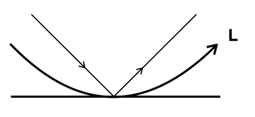 Figure 2: The contour L


