Hypertabastic survival models

Hypertabastic survival models were introduced in 2007 by Mohammad Tabatabai, Zoran Bursac, David Williams, and Karan Singh. This distribution can be used to analyze time-to-event data in biomedical and public health areas and normally called survival analysis. In engineering, the time-to-event analysis is referred to as reliability theory and in business and economics it is called duration analysis. Other fields may use different names for the same analysis. These survival models are applicable in many fields such as biomedical, behavioral science, social science, statistics, medicine, bioinformatics, medical informatics, data science especially in machine learning, computational biology, business economics, engineering, and commercial entities. They not only look at the time to event, but whether or not the event occurred. These time-to-event models can be applied in a variety of applications for instance, time after diagnosis of cancer until death, comparison of individualized treatment with standard care in cancer research, time until an individual defaults on loans, relapsed time for drug and smoking cessation, time until property sold after being put on the market, time until an individual upgrades to a new phone, time until job relocation, time until bones receive microscopic fractures when undergoing different stress levels, time from marriage until divorce, time until infection due to catheter, and time from bridge completion until first repair.

Hypertabastic cumulative distribution function

Illustration of Hypertabastic CDF for varying values of the beta parameter.

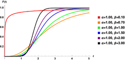
The Hypertabastic cumulative distribution function or simply the hypertabastic distribution function [math]\displaystyle{ F(t) }[/math] is defined as the probability that random variable [math]\displaystyle{ T }[/math] will take a value less than or equal to [math]\displaystyle{ t }[/math]. The hypertabastic distribution function is defined as

[math]\displaystyle{ F(t) = \begin{cases} 1 - \operatorname{sech}(\frac{\alpha(1-t^{\beta} \operatorname{coth}(t^{\beta}))}{\beta}) & t \gt 0 \\ 0 & t\leq 0 \end{cases} }[/math],

where [math]\displaystyle{ \operatorname{sech} }[/math] represents the hyperbolic secant function and [math]\displaystyle{ \alpha }[/math], [math]\displaystyle{ \beta }[/math] are parameters.

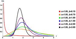
The parameters [math]\displaystyle{ \alpha }[/math] and [math]\displaystyle{ \beta }[/math] are both positive with [math]\displaystyle{ \operatorname{sech} }[/math] and [math]\displaystyle{ \operatorname{coth} }[/math] as hyperbolic secant and hyperbolic cotangent respectively. The Hypertabastic probability density function is

[math]\displaystyle{ f(t) = \begin{cases} \operatorname{sech}(W(t))(\alpha t^{2 \beta - 1}\operatorname{csch}^{2}(t^{\beta})-\alpha t^{\beta-1}\operatorname{coth}(t^{\beta}))\operatorname{tanh}(W(t))& t \gt 0 \\ 0 & t \lt 0 \end{cases} }[/math],

where [math]\displaystyle{ \operatorname{csch} }[/math] and [math]\displaystyle{ \operatorname{tanh} }[/math] are hyperbolic cosecant and hyperbolic tangent respectively and

[math]\displaystyle{ W(t)=\frac{\alpha(1-t^{\beta} \operatorname{coth}(t^{\beta}))}{\beta} }[/math]

Hypertabastic survival function

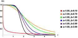
The Hypertabastic survival function is defined as

[math]\displaystyle{ S(t)=\operatorname{sech}[\frac{\alpha(1-t^\beta \operatorname{coth}(t^\beta))}{\beta}] }[/math],

where [math]\displaystyle{ S(t) }[/math] is the probability that waiting time exceeds [math]\displaystyle{ t }[/math].

For [math]\displaystyle{ t\gt 0 }[/math], the Restricted Expected (mean) Survival Time of the random variable [math]\displaystyle{ T }[/math] is denoted by [math]\displaystyle{ REST(t) }[/math], and is defined as

[math]\displaystyle{ REST(t)=\int_{0}^{t}{S(u)} du }[/math].

Hypertabastic hazard function

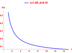
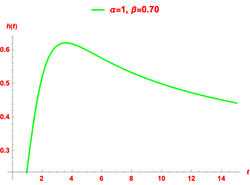
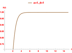
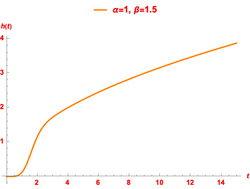
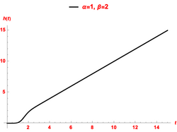
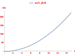
For the continuous random variable [math]\displaystyle{ T }[/math] representing time to event, the Hypertabastic hazard function [math]\displaystyle{ h(t) }[/math], which represents the instantaneous failure rate at time [math]\displaystyle{ t }[/math] given survival up to time [math]\displaystyle{ t }[/math], is defined as

[math]\displaystyle{ h(t) = \lim_{\Delta(t) \to 0^{+}} \frac{P(t \leq T \lt t + \Delta(t) | T \geq t)}{\Delta(t)}= \alpha (t^{2 \beta-1} \operatorname{csch}^{2} (t^{\beta}) -t^{\beta-1}\operatorname{coth} (t^{\beta})) \operatorname{tanh} (W(t)) }[/math].

The Hypertabastic hazard function has the flexibility to model varieties of hazard shapes. These different hazard shapes could apply to different mechanisms for which the hazard functions may not agree with conventional models. The following is a list of possible shapes for the Hypertabastic hazard function: For [math]\displaystyle{ 0 \lt \beta \leq 0.25 }[/math], the Hypertabastic hazard function is monotonically decreasing indicating higher likelihood of failure at early times. For [math]\displaystyle{ 0.25 \lt \beta \lt 1 }[/math], the Hypertabastic hazard curve first increases with time until it reaches its maximum failure rate and thereafter the failure decreases with time (unimodal). For [math]\displaystyle{ \beta = 1 }[/math], the Hypertabastic hazard function initially increases with time, then it reaches its horizontal asymptote [math]\displaystyle{ \alpha }[/math]. For [math]\displaystyle{ 1 \lt \beta \lt 2 }[/math], the Hypertabastic hazard function first increases with time with an upward concavity until it reaches its inflection point and subsequently continues to increase with a downward concavity. For [math]\displaystyle{ \beta = 2 }[/math], the Hypertabastic hazard function initially increases with an upward concavity until it reaches its point of inflection, thereafter becoming a linear asymptote with slope [math]\displaystyle{ \alpha }[/math]. For [math]\displaystyle{ \beta \gt 2 }[/math], the Hypertabastic hazard function increases with an upward concavity.

Hazard curves from the Hypertabastic distribution with varying beta parameter values.

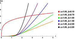
The Hypertabastic cumulative hazard function is

[math]\displaystyle{ H(t)= \int_{0}^{t}h(v)dv = -ln(S(t)) }[/math]

Hypertabastic proportional hazards model

The hazard function [math]\displaystyle{ h(t|\mathbf{x},\mathbf{\theta}) }[/math] of the Hypertabastic proportional hazards model has the form

[math]\displaystyle{ h(t|\mathbf{x},\mathbf{\theta})=h(t)g(\mathbf{\theta}|\mathbf{x}) }[/math],

where [math]\displaystyle{ \mathbf{x} }[/math] is a p-dimensional vector of explanatory variables and [math]\displaystyle{ \theta }[/math] is a vector of unknown parameters. The combined effect of explanatory variables [math]\displaystyle{ g(\mathbf{\theta}|\mathbf{x})= e^{-\theta_0 - \sum_{k=1}^{p}{\theta_kx_k}} }[/math] is a non-negative function of [math]\displaystyle{ x }[/math] with [math]\displaystyle{ g(\mathbf{\theta}|\mathbf{0})=e^{-\theta_0} }[/math]. The Hypertabastic survival function [math]\displaystyle{ S(t|\mathbf{x},\mathbf{\theta}) }[/math] for the proportional hazards model is defined as:

[math]\displaystyle{ S(t|\mathbf{x},\mathbf{\theta})=[S(t)]^{g(\mathbf{\theta}|\mathbf{x})} }[/math]

and the Hypertabastic probability density function for the proportional hazard model is given by

[math]\displaystyle{ f(t|\mathbf{x},\mathbf{\theta})=f(t)[S(t)]^{g(\mathbf{\theta}|\mathbf{x})-1}g(\mathbf{\theta}|\mathbf{x}) }[/math].

Depending on the type of censoring, the maximum likelihood function technique along with an appropriate log-likelihood function may be used to estimate the model parameters. If the sample consists of right censored data and the model to use is Hypertabastic proportional hazards model, then, the proportional hazards log-likelihood function is

[math]\displaystyle{ LL(\mathbf{\theta},\alpha,\beta:{\mathbf{x}})=\sum_{i=1}^{n}{(ln[{\operatorname{sech}(W(t_i))}]g(\mathbf{\theta}|\mathbf{x}_i)+\delta_i ln{[(\alpha {t_i}^{-1+2 \beta}\operatorname{csch}^{2}{({t_i}^{\beta})}-\alpha {t_i}^{-1+\beta}\operatorname{coth}({t_i}^{\beta}))\operatorname{tanh}(W(t_i))g(\mathbf{\theta}|\mathbf{x}_i)]})} }[/math].

Hypertabastic accelerated failure time model

When the covariates act multiplicatively on the time-scale, the model is called accelerated failure time model. The Hypertabastic survival function for the accelerated failure time model is given by

[math]\displaystyle{ S(t|\mathbf{x},\mathbf{\theta})=S(tg(\mathbf{\theta}|\mathbf{x})) }[/math].

The Hypertabastic accelerated failure time model has a hazard function [math]\displaystyle{ h(t|\mathbf{x},\mathbf{\theta}) }[/math] of the form

[math]\displaystyle{ h(t|\mathbf{x},\mathbf{\theta})=h(tg(\mathbf{\theta}|\mathbf{x}))g(\mathbf{\theta}|\mathbf{x}) }[/math].

The Hypertabastic probability density function for the accelerated failure time model is

[math]\displaystyle{ f(t|\mathbf{x},\mathbf{\theta})= f(tg(\mathbf{\theta}|\mathbf{x}))g(\mathbf{\theta}|\mathbf{x}) }[/math].

For the right censored data, the log-likelihood function for the Hypertabastic accelerated failure time model is given by

[math]\displaystyle{ LL(\mathbf{\theta},\alpha,\beta:{\mathbf{x}})=\sum_{i=1}^{n}{(ln{[\operatorname{sech}(\frac{\alpha{(Z(t_i))}^{\beta}\operatorname{coth}({Z(t_i)}^{\beta})}{\beta})]}+\delta_i ln{[(\alpha {(Z(t_i))}^{-1+2 \beta}\operatorname{csch}^{2}{[{Z(t_i)}^{\beta}]}-\alpha {Z(t_i)}^{\beta}\operatorname{tanh}(\frac{\alpha (1-{(Z(t_i))}^{\beta}\operatorname{coth}{(Z(t_i))}^\beta)}{\beta}))]}g(\mathbf{\theta}|\mathbf{x}_i))} }[/math],

where [math]\displaystyle{ Z(t_i) = t_i g(\mathbf{\theta}|\mathbf{x}_i) }[/math].

A modified chi-squared type test, known as Nikulin-Rao-Robson statistic is used to test the goodness-of-fit for Hypertabastic accelerated failure time models and its comparison with unimodal hazard rate functions. Simulation studies have shown that the Hypertabastic distribution can be used as an alternative to log-logistic and log-normal distribution because of its flexible shape of hazard functions. The Hypertabastic distribution is a competitor for statistical modeling when compared with Birnbaum-Saunders and inverse Gaussian distributions

Likelihood functions for survival analysis

Consider a sample of survival times of n individuals [math]\displaystyle{ t_1,t_2,\ldots,t_n }[/math] with associated p-dimensional covariate vectors [math]\displaystyle{ \mathbf{x}_1,\mathbf{x}_2,\ldots,\mathbf{x}_n }[/math] and an unknown parameter vector [math]\displaystyle{ \mathbf{\theta}=(\theta_0,\theta_1,\ldots,\theta_p) }[/math]. Let [math]\displaystyle{ f(t_i|\mathbf{x}_i,\mathbf{\theta}), F(t_i|\mathbf{x}_i,\theta), S(t_i|\mathbf{x}_i,) }[/math] and [math]\displaystyle{ h(t_i|\mathbf{x}_i,\mathbf{\theta}) }[/math] stand for the corresponding probability density function, cumulative distribution function, survival function and hazard function respectively. In the absence of censoring (censoring normally occurs when the failure time of some individuals cannot be observed), the likelihood function is

[math]\displaystyle{ L(\mathbf{\theta},\alpha,\beta:{\mathbf{x}})=\prod_{i=1}^{n}f(t_i|\mathbf{x}_i,\mathbf{\theta}) }[/math]

and the log-likelihood [math]\displaystyle{ LL(\mathbf{\theta},\alpha,\beta:{\mathbf{x}}) }[/math] is

[math]\displaystyle{ LL(\mathbf{\theta},\alpha,\beta:{\mathbf{x}})=\sum_{i=1}^{n}ln{[f(t_i|\mathbf{x}_i,\mathbf{\theta})]} }[/math]

For the right censored data, the likelihood function is

[math]\displaystyle{ L(\mathbf{\theta},\alpha,\beta:{\mathbf{x}})=\prod_{i=1}^{n}{[f(t_i|\mathbf{x}_i,\mathbf{\theta})]^{\delta_i}[S(t_i|\mathbf{x}_i,\mathbf{\theta})]^{1-\delta_i}} }[/math]

or equivalently,

[math]\displaystyle{ L(\mathbf{\theta},\alpha,\beta:{\mathbf{x}})=\prod_{i=1}^{n}{[h(t_i|\mathbf{x}_i,\mathbf{\theta})]^{\delta_i}S(t_i|\mathbf{x}_i,\mathbf{\theta})} }[/math],

and the log-likelihood function is

[math]\displaystyle{ LL(\mathbf{\theta},\alpha,\beta:{\mathbf{x}})=\sum_{i=1}^{n}(\delta_i ln{[f(t_i|\mathbf{x}_i,\mathbf{\theta})]}+(1-\delta_i) ln{[S(t_i|\mathbf{x}_i,\mathbf{\theta})]}) }[/math]

or equivalently,

[math]\displaystyle{ LL(\mathbf{\theta},\alpha,\beta:{\mathbf{x}})=\sum_{i=1}^{n}(\delta_i ln{[h(t_i|\mathbf{x}_i,\mathbf{\theta}]}+ln{[S(t_i|\mathbf{x}_i,\mathbf{\theta})]}) }[/math]

where

[math]\displaystyle{ \delta_i = \begin{cases} 0 & t_i \text{is a right censored observation} \\ 1 & otherwise \end{cases} }[/math],

In the presence of left censored data, the likelihood function is

[math]\displaystyle{ L(\mathbf{\theta},\alpha,\beta:{\mathbf{x}})=\prod_{i=1}^{n}[f(t_i|\mathbf{x}_i,\mathbf{\theta})]^{\gamma_i}[F(t_i|\mathbf{x}_i,\mathbf{\theta})]^{1-\gamma_i} }[/math]

and the corresponding log-likelihood function is

[math]\displaystyle{ LL(\mathbf{\theta},\alpha,\beta:{\mathbf{x}})=\sum_{i=1}^{n}(\gamma_i ln{[f(t_i|\mathbf{x}_i,\mathbf{\theta})]}+(1-\gamma_i)ln{[F(t_i|\mathbf{x}_i,\mathbf{\theta})]}) }[/math]

where

[math]\displaystyle{ \gamma_i = \begin{cases} 0 & t_i \text{is a left censored observation} \\ 1 & otherwise \end{cases} }[/math],

In the presence of interval censored data, the likelihood function is

[math]\displaystyle{ L(\mathbf{\theta},\alpha,\beta:{\mathbf{x}})=\prod_{i=1}^{n}([f(t_i|\mathbf{x}_i,\mathbf{\theta})]^{\xi_i}[F(v_i|\mathbf{x}_i,\mathbf{\theta})-F(u_i|\mathbf{x}_i,\mathbf{\theta})]^{1-\xi_i}) }[/math]

and the log-likelihood function is

[math]\displaystyle{ LL(\mathbf{\theta},\alpha,\beta:{\mathbf{x}})=\sum_{i=1}^{n}(\xi_i ln{[f(t_i|\mathbf{x}_i,\mathbf{\theta})]}+(1-\xi_i) ln{[F(v_i|\mathbf{x}_i,\mathbf{\theta})-F(u_i|\mathbf{x}_i,\mathbf{\theta})]}) }[/math]

where [math]\displaystyle{ u_i \le t_i \le v_i }[/math] for all interval censored observations and

[math]\displaystyle{ \xi_i = \begin{cases} 0 & t_i \text{is an interval censored observation} \\ 1 & otherwise \end{cases} }[/math],

If the intended sample consists of all types of censored data (right censored, left censored and interval censored), then its likelihood function takes the following form

[math]\displaystyle{ L(\mathbf{\theta},\alpha,\beta:{\mathbf{x}})=\prod_{i=1}^{n}([S(t_i|\mathbf{x}_i,\mathbf{\theta})]^{1-\delta_i}[F(t_i|\mathbf{x}_i,\mathbf{\theta})]^{1-\gamma_i}[F(v_i|\mathbf{x}_i,\mathbf{\theta})-F(u_i|\mathbf{x}_i,\mathbf{\theta})]^{1-\xi_i}[f(t_i|\mathbf{x}_i,\mathbf{\theta})]^{\delta_i+\gamma_i+\xi_i-2}) }[/math]

and its corresponding log-likelihood function is given by

[math]\displaystyle{ LL(\mathbf{\theta},\alpha,\beta:{\mathbf{x}})=\sum_{i=1}^{n}{(1-\delta_i) ln{[S(t_i|\mathbf{x}_i,\mathbf{\theta})]}+(1-\gamma_i)ln{[F(t_i|\mathbf{x}_i,\mathbf{\theta})]}(1-\xi_i)ln{[F(v_i|\mathbf{x}_i,\mathbf{\theta})-F(u_i|\mathbf{x}_i,\mathbf{\theta})]}+ (\delta_i+\gamma_i+\xi_i-2)ln{[f(t_i|\mathbf{x}_i,\mathbf{\theta})]}} }[/math]

Applications of hypertabastic survival models

Cutaneous or mucosal melanoma

The Hypertabastic Accelerated Failure Time model was used to analyze a total of 27,532 patients regarding the impact of histology on the survival of patients with cutaneous or mucosal melanoma. Understanding patients’ histological subtypes and their failure rate assessment would enable clinicians and healthcare providers to perform individualized treatment, resulting in a lower risk of complication and higher survivability of patients.

Oil field quantities

The quantities of 49 locations of the same area of an oil field was examined to identify its underlying distribution. Using generalized chi-squared, the distribution of oil field quantities was represented by the Hyperbolastic distribution and compared with the lognormal (LN), log-logistic (LL), Birnbaum-Saunders (BS) and inverse Gaussian (IG) distributions.

Remission duration for acute leukemia

The times of remission from clinical trial for acute leukemia of children study were used to analyze the remission duration of acute leukemia data for two groups of patients controlling for log of white blood cell counts. The Hypertabastic accelerated failure time model was used to analyze the remission duration of acute leukemia patient.

Brain tumor study of malignant glioma patients

A randomized clinical trial comparing two chemotherapy regimens for 447 individuals with malignant glioma. A total of 293 patients died within a five-year time period and the median survival time was about 11 months. The overall model fit, in comparison with other parametric distributions, was performed using the generalized chi-square test statistics and proportional hazards model.

Analysis of breast cancer patients

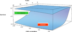
The Hypertabastic proportional hazard model was used to analyze numerous breast cancer data including the survival of breast cancer patients by exploring the role of a metastasis variable in combination with clinical and gene expression variables.

Analysis of hypertensive patients

One hundred five Nigerian patients who were diagnosed with hypertension from January 2013 to July 2018 were included in this study, where death was the event of interest. Six parametric models such as; exponential, Weibull, lognormal, log-logistic, Gompertz and Hypertabastic distributions were fitted to the data using goodness of fit tests such as S.E., AIC, and BIC to determine the best fit model. The parametric models were considered because they are all lifetime distributions. S.E., AIC, and BIC measures were used to compare these parametric models.

Analysis of cortical bone fracture

Stress fractures in older individuals are very important due to the growing number of elderly. Fatigue tests on 23 female bone samples from three individuals were analyzed. Hypertabastic survival and hazard functions of the normalized stress level and age were developed using previously published bone fatigue stress data. The event of interest was the number of cycles until the bone gets microscopic fracture. Furthermore, Hypertabastic proportional hazard models were used to investigate tensile fatigue and cycle-to-fatigue for cortical bone data.

Analysis of unemployment

Hypertabastic survival models have been used in the analysis of unemployment data and its comparison with the cox regression model.

Analysis of kidney carcinoma patients

3-D model of hazard curves of various kidney carcinoma histological subtypes.

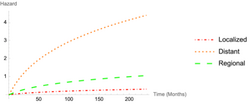
Using National Cancer Institute data from 1975 to 2016, the impact of histological subtypes on the survival probability of 134,150 kidney carcinoma patients were examined. The study variables were a race/ethnicity, age, sex, tumor grade, type of surgery, geographical location of patient and stage of disease. The Hypertabastic proportional hazards model was used to analyze the survival time of patients diagnosed with kidney carcinoma to explore the effect of histological subtypes on their survival probability and assess the relationship between the histological subtypes, tumor stage, tumor grade, and type of surgery.

Kidney carcinoma SAS example code

Sample code in SAS:

Proc nlp data=sasuser.KidneyCarcinoma tech=quanew cov=2 vardef=n pcov phes maxiter=250; 
  /* Hypertabastic Proportional Hazards Model with Log Time */ 
  title1 'Kidney Carcinoma';
  max logf; 
  
  /* Model Parameter Initial Values for Explanatory Variables */
  parms a=0.01,b=0.1, 
  c=0.01, /* Age */ /* Continuous */
  d=-.01, /* Male */ /* reference: Female */
  r1=.071, /* Hispanic */
  r2=.044, /* Asian */
  r3=.134, /* Black */ /* reference: White */
  h1=.205, /* Adeno Carcinoma w/ Mixed Subtypes */
  h2=.505, /* Papillary Adeno Carcinoma NOS */
  h3=.537, /* Clear Cell Adeno Carcinoma */
  h4=.316, /* Renal Cell Adeno Carcinoma */
  h5=1.15, /* Chromophobe Renal Cell Carcinoma */
  h6=-.21, /* Sarcomatoid Renal Cell Carcinoma */
  h7=.378, /* Granular Cell Carcinoma */ /* reference: Other */
  g1=.03, /* East */ 
  g2=.088, /* Northern Plains */ 
  g3=.06, /* Pacific Coast */ /* reference: Southwest */
  s1=1.2, /* Localized */
  s2=-1.3, /* Distant */ /* reference: Regional */
  gr1=1.169, /* Well Differentiated */
  gr2=.99, /* Moderately Differentiated */
  gr3=.413, /* Poorly Differentiated */ /* reference: Undifferentiated */
  su1=-.945, /* No Surgery */
  su2=.84, /* Cryocergery */
  su3=.56, /* Thermal Ablation */
  su4=.574, /* Cryosurgery */
  su5=1.173, /* Partial Nephrectomy or Partial Uretterectomy */
  su6=.25, /* Complete Nephrectomy */
  su7=.073, /* Radical Nephrectomy */
  su8=-.096, /* Any Nephrectomy */
  su9=.028; /* Nephrectomy, Urectomy */ /* reference: Other */
  
  /* Log-Likelihood Function */ 
  in6=exp(-(c*Age+
  d*Gender+
  r1*Race1+r2*Race2+r3*Race3+
  h1*Hist1+h2*Hist2+h3*Hist3+h4*Hist4+h5*Hist5+h6*Hist6+h7*Hist7+
  g1*Geo1+g2*Geo2+g3*Geo3+
  s1*Stage1+s2*Stage2+
  gr1*Grade1+gr2*Grade2+gr3*Grade3+
  su1*Surgery1+su2*Surgery2+su3*Surgery3+su4*Surgery4+su5*Surgery5+su6*Surgery6+su7*Surgery7+su8*Surgery8+su9*Surgery9)); /* covariates */ 
  
  s = log(1/cosh(a*(1-(time**b)/tanh(time**b))/b))*in6+Status*log(((a*time**(-1+2*b)/sinh(time**b)**2-
  a*time**(-1+b)/tanh(time**b))*tanh(a*(1-time**b/tanh(time**b))/b))*in6);
  
  logf=s;
run;

Applications of hypertabastic survival models in bridge engineering

Defines points of interest on a bridge deck superstructure.

Although survival analysis tools and techniques have been widely used in medical and biomedical applications over the last few decades, their applications to engineering problems have been more sporadic and limited. The probabilistic assessment of service life of a wide variety of engineering systems, from small mechanical components to large bridge structures, can substantially benefit from the well-established survival analysis techniques. Modeling of time-to-event phenomena in engineering applications can be performed under the influence of numerical and categorical covariates using observational or test data. The "survival" of an engineering component or system is synonymous with the more commonly used term "reliability". The term "hazard rate" or "conditional failure rate" (defined as probability of survival per unit time assuming survival up to that time) is an important measure of the change in the rate of failure over time. In this context, failure is defined as reaching the target event in the time-to-event process. This could be defined as reaching a particular serviceability condition state, localized/partial structural failure, or global/catastrophic failure applied the Hypertabastic parametric accelerated failure time survival model to develop probabilistic models of bridge deck service life for Wisconsin. Bridge decks are typically concrete slabs on which traffic rides as seen in the Marquette Interchange bridge. The authors used the National Bridge Inventory (NBI) dataset to obtain the needed data for their study. NBI records include discrete numerical ratings for bridge decks (and other bridge components) as well as other basic information such as Average Daily Traffic (ADT) and deck surface area (obtained by multiplying the provided bridge length with bridge deck width). The numerical ratings range from 0 to 9 with 9 corresponding to brand new condition and 0 being complete failure. A deck condition rating of 5 was selected as the effective end of service life of bridge deck. The numerical covariates used were the ADT and deck surface area, while the categorical covariate was the superstructure material (structural steel or concrete).

The hypertabastic Proportional Hazards and Accelerated Failure Time models are useful techniques in analyzing bridge-related structures due to its flexibility of hazard curves, which can be monotonically increasing or decreasing with upward or downward concavity. It can also take the shape of a single mound curve. This flexibility in modeling various hazard shapes makes the model suitable for a wide variety of engineering problems.

Tabatabai et al. extended the Hypertabastic bridge deck models developed for Wisconsin bridges to bridges in six northern US states Nabizadeh, A. (2015). Reliability of Bridge Superstructures in Wisconsin. Master's Thesis (Thesis). UWM Digital Commons. and then to all 50 US states. The study of bridge decks in all 50 states indicated important differences in reliability of bridge decks in different states and regions. Stevens et al. discuss the importance of survival analyses in identifying key bridge performance indicators and discuss the use of Hypertabastic survival models for bridges. and Nabizadeh et al. further extended the use of Hypertabastic survival models to bridge superstructures. The covariates used were ADT, maximum bridge span length and superstructure type. The survival function can be used to determine the expected life using the following equation (area under the entire survival curve)

[math]\displaystyle{ {EL}_0=\int_{0}^{\infty}S(t)dt }[/math]

It is important to note that both the survival function and the expected life would change as the time passes by. The conditional survival function [math]\displaystyle{ C_S }[/math] is a function of time [math]\displaystyle{ t }[/math] and survival time [math]\displaystyle{ t_s }[/math] and is defined as

[math]\displaystyle{ CS(t,t_s) = \begin{cases} 1 & 0 \le t \le t_s \\ \frac{S(t)}{S(t_s)} & t \gt t_s \end{cases} }[/math],

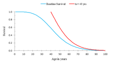
Nabizadeh et al. used the Hypertabastic survival functions developed for Wisconsin to analyze conditional survival functions and conditional expected service lives [math]\displaystyle{ (EL_c(t_s)) }[/math]

[math]\displaystyle{ {EL}_c(t_s)=\int_{0}^{\infty}CS(t)dt=t_s+\int_{t_s}^{\infty}{CS(t)dt=t_s+\int_{t_s}^{\infty}\frac{S(t)}{S(t_s)}}dt }[/math]

The conditional expected life would continue to increase as the survival time [math]\displaystyle{ t_s }[/math] increases. Nabizadeh et al. term this additional expected life as "survival dividend.”

An important mode of failure in bridge engineering is metal fatigue, which can result from repetitive applications of stress cycles to various details and connections in the structure. As the number of cycles [math]\displaystyle{ (n_c) }[/math] increase, the probability of fatigue failure increases. An important factor in fatigue life [math]\displaystyle{ (N_c) }[/math] is the stress range (Sr)(maximum minus minimum stress in a cycle). The probabilistic engineering fatigue problem can be treated as a "time"-to-event survival analysis problem if the number of cycles [math]\displaystyle{ (n_c) }[/math] is treated as a fictitious time variable [math]\displaystyle{ (t) }[/math]

This would facilitate the application of well-established survival analysis techniques to engineering fatigue problems and Tabatabai et al. The survival function [math]\displaystyle{ S(n_c) }[/math], probability density function [math]\displaystyle{ f(n_c) }[/math], hazard rate [math]\displaystyle{ h(n_c) }[/math], and cumulative probability of failure [math]\displaystyle{ F(n_c) }[/math] can then be defined as

[math]\displaystyle{ S(n_c)=P(N_c\gt n_c)=1-F(n_c) }[/math]

[math]\displaystyle{ f(n_c)=\lim_{\delta n_c \to 0} \frac{P(n_c\lt N_c\lt n_c+\delta n_c)}{\delta n_c} }[/math]

[math]\displaystyle{ h(n_c)=\lim_{\delta n_c \to 0} \frac{P(n_c\lt N_c\lt n_c+\delta n_c| N_c\gt n_c)}{\delta n_c} }[/math]

The hypertabastic accelerated failure time model was used to analyze probabilistic fatigue life for various detailed categories in steel bridges.

References

- ↑ 1.0 1.1 Tabatabai, Mohammad A.; Bursac, Zoran; Williams, David K.; Singh, Karan P. (2007). "Hypertabastic survival model". Theoretical Biology and Medical Modelling 4 (40): 40. doi:10.1186/1742-4682-4-40. PMID 17963492.
- ↑ 2.0 2.1 Tahir, M Ramzan; Tran, Quang X; Nikulin, Mikhail S (2017). "Comparison of hypertabastic survival model with other unimodal hazard rate functions using a goodness-of-fit test". Statistics in Medicine 36 (12): 1936–1945. doi:10.1002/sim.7244. PMID 28173610.
- ↑ Nikulin, Mikhail; Wu, Hong-Dar Isaac (2016). The Cox Model and Its Applications. Springer. ISBN 978-3-662-49332-8.
- ↑ Singh, K. P.; Nsetan, H. N. (2019). "A flexilble family of hypertabastic models". 23rd International Congress on Modelling and Simulation. Canberra, ACT, Australia. https://mssanz.org.au/modsim2019/I1/singh.pdf.
- ↑ M.A., Hayat (2014). Stem Cells and Cancer Stem Cells Volume 12. Springer. ISBN 978-94-017-8032-2.
- ↑ Cleophas, T.J.; Zwinderman, A.H. (2023). Modern Survival Analysis in Clinical Research. Springer. ISBN 978-3-031-31631-9.
- ↑ Tabatabai, Mohammad A. (2023). "The role of histological subtypes in the survival of patients diagnosed with cutaneous or mucosal melanoma in the United States of America". PLOS ONE 18 (6). doi:10.1371/journal.pone.0286538. PMID 37276224.
- ↑ 8.0 8.1 8.2 Tran, Xuan Quang (2015). Dynamic regression models and their applications in survival and reliability analysis (Thesis). HAL archives-ouvertes.fr.
- ↑ Tabatabai, Mohammad A.; Eby, Wayne M.; Nimeh, Nadim (2012). "Role of Metastasis in Hypertabastic Survival Analysis of Breast Cancer: Interaction with Clinical and Gene Expression Variables". Cancer Growth and Metastasis 5. doi:10.4137/CGM.S8821.
- ↑ Tabatabai, Mohammad A.; Eby, Wayne M.; Nimeh, Nadim (2012). "Clinical and multiple gene expression variables in survival analysis of breast cancer: Analysis with the hypertabastic survival model". BMC Medical Genomics 5. doi:10.1186/1755-8794-5-63. PMID 23241496.
- ↑ Ibenegbu, Amuche Henrietta; Osuji, George Amaeze; Edith Uzoma, Umeh (2020). "Comparison of Parametric Models: Application to Hypertensive Patients in a Teaching Hospital, Awka". Journal of Biostatistics and Epidemiology. ISSN 2383-4196.
- ↑ Tabatabai, Mohammad; Bae, Sejong; Singh, K. P. (2015). "Analysis of Survival Data Using Hypertabastic Models". 60th World Statistics Congress. Rio De Janeiro, Brazil. https://2015.isiproceedings.org/Files/CPS473-P1-A.pdf.
- ↑ Himali, L.P.; Xia, Zhiming (2022). "Performance of the Survival models in Socioeconomic Phenomena". Vavuniya Journal of Science 1 (2): 9–19. doi:10.4038/vjs.v1i2.9. ISSN 2950-7154.
- ↑ Tabatabai, Mohammad; Bailey, Stephanie; Matthews-Juarez, Patricia; Tabatabai, Habib (2020). "A Comprehensive Analysis of the Effect of Histological Subtypes on the Survival Probability of Kidney Carcinoma Patients: A Hypertabastic Survival Analysis". Journal of Renal Cancer 3 (1): 20–33. doi:10.36959/896/604. PMID 20953843.
- ↑ Tabatabai, Habib; Nabizadeh, Azam; Tabatabai, Mohammad; Tabatabai, Habib (2018). "Overview of Survival Analysis Techniques for Probabilistic Assessment of Bridge Service Life". Proceedings of Structural Faults and Repair Conference. Edinburgh, UK. doi:10.25084/ebridge.2018.0010.
- ↑ 16.0 16.1 16.2 Tabatabai, H.; Tabatabai, M.A.; Lee, C.W. (2011). "Reliability of Bridge Decks in Wisconsin". Journal of Bridge Engineering 16 (1): 53–62. doi:10.1061/(ASCE)BE.1943-5592.0000133.
- ↑ Bursac, Z.; Tabatabai, M.; Williams, D.K. (2008). "A simulation study of performance of hypertabastic and hyperbolastic survival models in comparison with classic survival models". 617–622.
- ↑ Tabatabai, H.; Lee, C.W.; Tabatabai, M.A. (2015). "Reliability of Bridge Decks in the United States". Bridge Structures 11 (3): 75–85. doi:10.3233/BRS-150091.
- ↑ Stevens, N.A.; Lydon, M.; Marshall, A.H. (2020). "Identification of Bridge Key Performance Indicators Using Survival Analysis for Future Network-Wide Structural Health Monitoring". Sensors 20 (23): 6894. doi:10.3390/s20236894. PMID 33276606. Bibcode: 2020Senso..20.6894S.
- ↑ Nabizadeh, A. (2015). Reliability of Bridge Superstructures in Wisconsin. Master's Thesis (Thesis). UWM Digital Commons.
- ↑ Nabizadeh, A.; Tabatabai, H.; Tabatabai, M.A. (2018). "Survival Analysis of Bridge Superstructures in Wisconsin". Applied Sciences 8 (11): 2079. doi:10.3390/app8112079.
- ↑ 22.0 22.1 Nabizadeh, A.; Tabatabai, H.; Tabatabai, M.A. (2020). "Conditional Survival Analysis for Concrete Bridge Decks". Life Cycle Reliability and Safety Engineering 9: 63–75. doi:10.1007/s41872-019-00100-4.
- ↑ 23.0 23.1 23.2 Nabizadeh, A.; Tabatabai, H. (2020). "Development of nonlinear probabilistic S–N curves using survival analysis". International Journal of Fatigue 141. doi:10.1016/j.ijfatigue.2020.105892.
- ↑ Tabatabai, H.; Nabizadeh, A.; Tabatabai, M.A. (2019). "Survival Analysis Approach for Fatigue Reliability Assessment in Bridge Structures". Proceedings of BEI-2019 conference, Bridge Engineering Institute (BEI). Honolulu, Hawaii, US. https://mssanz.org.au/modsim2019/I1/singh.pdf.