Multifidelity simulation
 Multifidelity Simulation Methods for Transportation[1] | |
| Class | |
|---|---|
| Data structure | Low- and high-fidelity data |
| Worst-case performance | Not defined |
| Worst-case space complexity | Not defined |
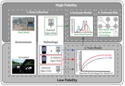
Multifidelity (or multi-fidelity) methods leverage both low- and high-fidelity data in order to maximize the accuracy of model estimates, while minimizing the cost associated with parametrization. They have been successfully used in impedance cardiography,[2][3][4] wing-design optimization,[5] robotic learning,[6] computational biomechanics,[7] and have more recently been extended to human-in-the-loop systems, such as aerospace[8] and transportation.[9] They include both model-based methods, where a generative model is available or can be learned, in addition to model-free methods, that include regression-based approaches, such as stacked-regression.[8] A more general class of regression-based multi-fidelity methods are Bayesian approaches, e.g. Bayesian linear regression,[3] Gaussian mixture models,[10][11] Gaussian processes,[12] auto-regressive Gaussian processes,[2] or Bayesian polynomial chaos expansions.[4]
The approach used depends on the domain and properties of the data available, and is similar to the concept of metasynthesis, proposed by Judea Pearl.[13]
Data fidelity spectrum

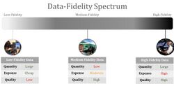
The fidelity of data can vary along a spectrum between low- and high-fidelity. The next sections provide examples of data across the fidelity spectrum, while defining the benefits and limitations of each type of data.
Low fidelity data (LoFi)
Low-fidelity data (LoFi) includes any data that was produced by a person or Stochastic Process that deviates from the real-world system of interest. For example, LoFi data can be produced by models of a physical system that use approximations to simulate the system, rather than modeling the system in an exhaustive manner.[5]
Moreover, in human-in-the-loop (HITL) situations the goal may be to predict the impact of technology on expert behavior within the real-world operational context. Machine learning can be used to train statistical models that predict expert behavior, provided that an adequate amount of high-fidelity (i.e., real-world) data are available or can be produced.[8]
LoFi benefits and limitations
In situations when there is not an adequate amount of high-fidelity data available to train the model, low-fidelity data can sometimes be used. For example, low-fidelity data can be acquired by using a distributed simulation platform, such as X-Plane, and requiring novice participants to operate in scenarios that are approximations of the real-world context. The benefit of using low-fidelity data is that they are relatively inexpensive to acquire, so it is possible to elicit larger amounts of data. However, the limitation is that the low-fidelity data may not be useful for predicting real-world expert (i.e., high-fidelity) performance due to differences between the low-fidelity simulation platform and the real-world context, or between novice and expert performance (e.g., due to training).[8][9]
High-fidelity data (HiFi)
High-fidelity data (HiFi) includes data that was produced by a person or Stochastic Process that closely matches the operational context of interest. For example, in wing design optimization, high-fidelity data uses physical models in simulation that produce results that closely match the wing in a similar real-world setting.[5] In HITL situations, HiFi data would be produced from an operational expert acting in the technological and situational context of interest.[9]
HiFi benefits and limitations
An obvious benefit of utilizing high-fidelity data is that the estimates produced by the model should generalize well to the real-world context. However, these data are expensive in terms of both time and money, which limits the amount of data that can be obtained. The limited amount of data available can significantly impair the ability of the model to produce valid estimates.[8]
Multifidelity methods (MfM)
Multifidelity methods attempt to leverage the strengths of each data source, while overcoming the limitations. Although small to medium differences between low- and high-fidelity data are sometimes able to be overcome by multifidelity models, large differences (e.g., in KL divergence between novice and expert action distributions) can be problematic leading to decreased predictive performance when compared to models that exclusively relied on high-fidelity data.[8]
Multifidelity models enable low-fidelity data to be collected on different technology concepts to evaluate the risk associated with each concept before actually deploying the system.[14]
Bayesian auto-regressive Gaussian processes
In an auto-regressive model of Gaussian processes (GP), each level of output fidelity, , where a higher denotes a higher fidelity, is modeled as a GP, ,[15][2] which can be expressed in terms of the previous level's GP, , a proportionality constant and a "difference-GP" as follows:
The scaling constant that quantifies the correlation of levels and , and can generally depend on .[16][17]
Under the assumption, that all information about a level is contained in the data corresponding to the same pivot point at level as well as , semi-analytical first and second moments are feasible. This assumption formally is
I.e. given a data at on level , there is no further information about level to extract from the data on level .
References
- ↑ 1.0 1.1 Erik J. Schlicht (2017). "SAMSI Summer Program on Transportation Statistics: Erik Schlicht, Aug 15, 2017". Using Multifidelity Methods to Estimate the Risk Associated with Transportation Systems. https://www.samsi.info/news-and-media/summer-program-on-transportation-statistics-erik-schlicht-aug-15-2017/.
- ↑ 2.0 2.1 2.2 Ranftl, Sascha; Melito, Gian Marco; Badeli, Vahid; Reinbacher-Köstinger, Alice; Ellermann, Katrin; von der Linden, Wolfgang (2019-12-31). "Bayesian Uncertainty Quantification with Multi-Fidelity Data and Gaussian Processes for Impedance Cardiography of Aortic Dissection". Entropy 22 (1): 58. doi:10.3390/e22010058. ISSN 1099-4300. PMID 33285833. Bibcode: 2019Entrp..22...58R.
- ↑ 3.0 3.1 Ranftl, Sascha; Melito, Gian Marco; Badeli, Vahid; Reinbacher-Köstinger, Alice; Ellermann, Katrin; Linden, Wolfgang von der (2019-12-09). "On the Diagnosis of Aortic Dissection with Impedance Cardiography: A Bayesian Feasibility Study Framework with Multi-Fidelity Simulation Data". Proceedings 33 (1): 24. doi:10.3390/proceedings2019033024. ISSN 2504-3900.
- ↑ 4.0 4.1 Badeli, Vahid; Ranftl, Sascha; Melito, Gian Marco; Reinbacher-Köstinger, Alice; Von Der Linden, Wolfgang; Ellermann, Katrin; Biro, Oszkar (2021-01-01). "Bayesian inference of multi-sensors impedance cardiography for detection of aortic dissection". COMPEL - the International Journal for Computation and Mathematics in Electrical and Electronic Engineering 41 (3): 824–839. doi:10.1108/COMPEL-03-2021-0072. ISSN 0332-1649. https://doi.org/10.1108/COMPEL-03-2021-0072.
- ↑ 5.0 5.1 5.2 Robinson, T.D.; et, al (2006). "Multifidelity Optimization for Variable-Complexity Design". 11th AIAA/ISSMO Multidisciplinary Analysis and Optimization Conference: 1–18.
- ↑ Cutler, M.; et, al (2015). "Real-world reinforcement learning via multifidelity simulators.". IEEE Transactions on Robotics 31 (3): 655–671. doi:10.1109/TRO.2015.2419431.
- ↑ Sajjadinia, Seyed Shayan; Carpentieri, Bruno; Shriram, Duraisamy; Holzapfel, Gerhard A. (2022-09-01). "Multi-fidelity surrogate modeling through hybrid machine learning for biomechanical and finite element analysis of soft tissues" (in en). Computers in Biology and Medicine 148: 105699. doi:10.1016/j.compbiomed.2022.105699. ISSN 0010-4825. https://www.sciencedirect.com/science/article/pii/S0010482522004796.
- ↑ 8.0 8.1 8.2 8.3 8.4 8.5 Schlicht, Erik (2014). "Predicting the behavior of interacting humans by fusing data from multiple sources". arXiv:1408.2053 [cs.AI].
- ↑ 9.0 9.1 9.2 Schlicht, Erik J; Morris, Nichole L (2017). "Estimating the risk associated with transportation technology using multifidelity simulation". arXiv:1701.08588 [stat.AP].
- ↑ Koutsourelakis, Phaedon-Stelios (January 2009). "Accurate Uncertainty Quantification Using Inaccurate Computational Models" (in en). SIAM Journal on Scientific Computing 31 (5): 3274–3300. doi:10.1137/080733565. ISSN 1064-8275. http://epubs.siam.org/doi/10.1137/080733565.
- ↑ Biehler, Jonas; Gee, Michael W.; Wall, Wolfgang A. (2015-06-01). "Towards efficient uncertainty quantification in complex and large-scale biomechanical problems based on a Bayesian multi-fidelity scheme" (in en). Biomechanics and Modeling in Mechanobiology 14 (3): 489–513. doi:10.1007/s10237-014-0618-0. ISSN 1617-7940. PMID 25245816. https://doi.org/10.1007/s10237-014-0618-0.
- ↑ Nitzler, Jonas; Biehler, Jonas; Fehn, Niklas; Koutsourelakis, Phaedon-Stelios; Wall, Wolfgang A. (2020-01-09). "A Generalized Probabilistic Learning Approach for Multi-Fidelity Uncertainty Propagation in Complex Physical Simulations". arXiv:2001.02892 [cs.CE].
- ↑ Judea Pearl (2012). "The Do-Calculus Revisited". Proceedings of the Twenty-Eighth Conference on Uncertainty in Artificial Intelligence. Corvallis, OR: AUAI Press. pp. 4–11. https://pdfs.semanticscholar.org/2aa1/546b3a935a7876d9e7dbc764a92f0a29074d.pdf.
- ↑ Reshama Shaikh and Erik J. Schlicht (2017). "The Machine Learning Conference Interview with Dr. Schlicht". Interview Regarding the use of Multifidelity Simulation Methods. https://mlconf.com/interview-erik-schlicht-founder-computational-cognition-group-c2-g-llc-reshama-shaikh/.
- ↑ Kennedy, M. (2000-03-01). "Predicting the output from a complex computer code when fast approximations are available". Biometrika 87 (1): 1–13. doi:10.1093/biomet/87.1.1. ISSN 0006-3444. https://doi.org/10.1093/biomet/87.1.1.
- ↑ Parussini, L.; Venturi, D.; Perdikaris, P.; Karniadakis, G.E. (May 2017). "Multi-fidelity Gaussian process regression for prediction of random fields" (in en). Journal of Computational Physics 336: 36–50. doi:10.1016/j.jcp.2017.01.047. Bibcode: 2017JCoPh.336...36P. https://linkinghub.elsevier.com/retrieve/pii/S0021999117300633.
- ↑ Le Gratiet, Loic; Garnier, Josselin (2014). "Recursive Co-Kriging Model for Design of Computer Experiments with Multiple Levels of Fidelity" (in en). International Journal for Uncertainty Quantification 4 (5): 365–386. doi:10.1615/Int.J.UncertaintyQuantification.2014006914. ISSN 2152-5080. http://www.dl.begellhouse.com/journals/52034eb04b657aea,2f7b99cc281f2702,4c83626c5e64207a.html.
 |
