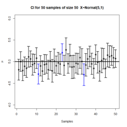
Neyman construction

Neyman construction, named after Jerzy Neyman, is a frequentist method to construct an interval at a confidence level [math]\displaystyle{ C, \, }[/math] such that if we repeat the experiment many times the interval will contain the true value of some parameter a fraction [math]\displaystyle{ C\, }[/math] of the time.

Theory

Assume [math]\displaystyle{ X_{1},X_{2},...X_{n} }[/math] are random variables with joint pdf [math]\displaystyle{ f(x_{1},x_{2},...x_{n} | \theta_{1},\theta_{2},...,\theta_{k}) }[/math], which depends on k unknown parameters. For convenience, let [math]\displaystyle{ \Theta }[/math] be the sample space defined by the n random variables and subsequently define a sample point in the sample space as [math]\displaystyle{ X=(X_{1},X_{2},...X_{n}) }[/math]
Neyman originally proposed defining two functions [math]\displaystyle{ L(x) }[/math] and [math]\displaystyle{ U(x) }[/math] such that for any sample point,[math]\displaystyle{ X }[/math],

• [math]\displaystyle{ L(X)\leq U(X) }[/math] [math]\displaystyle{ \forall X\in\Theta }[/math]
• L and U are single valued and defined.

Given an observation, [math]\displaystyle{ X^' }[/math], the probability that [math]\displaystyle{ \theta_{1} }[/math] lies between [math]\displaystyle{ L(X^') }[/math] and [math]\displaystyle{ U(X^') }[/math] is defined as [math]\displaystyle{ P(L(X^')\leq\theta_{1}\leq U(X^') | X^') }[/math] with probability of [math]\displaystyle{ 0 }[/math] or [math]\displaystyle{ 1 }[/math]. These calculated probabilities fail to draw meaningful inference about [math]\displaystyle{ \theta_{1} }[/math] since the probability is simply zero or unity. Furthermore, under the frequentist construct the model parameters are unknown constants and not permitted to be random variables. For example if [math]\displaystyle{ \theta_{1}=5 }[/math], then [math]\displaystyle{ P(2 \leq 5\leq 10)=1 }[/math]. Likewise, if [math]\displaystyle{ \theta_{1}=11 }[/math], then [math]\displaystyle{ P(2 \leq 11 \leq 10)=0 }[/math]

As Neyman describes in his 1937 paper, suppose that we consider all points in the sample space, that is, [math]\displaystyle{ \forall X\in\Theta }[/math], which are a system of random variables defined by the joint pdf described above. Since [math]\displaystyle{ L }[/math] and [math]\displaystyle{ U }[/math] are functions of [math]\displaystyle{ X }[/math] they too are random variables and one can examine the meaning of the following probability statement:

Under the frequentist construct the model parameters are unknown constants and not permitted to be random variables. Considering all the sample points in the sample space as random variables defined by the joint pdf above, that is all [math]\displaystyle{ X\in\Theta }[/math] it can be shown that [math]\displaystyle{ L }[/math] and [math]\displaystyle{ U }[/math] are functions of random variables and hence random variables. Therefore one can look at the probability of [math]\displaystyle{ L(X) }[/math] and [math]\displaystyle{ U(X) }[/math] for some [math]\displaystyle{ X\in\Theta }[/math]. If [math]\displaystyle{ \theta_{1}^' }[/math] is the true value of [math]\displaystyle{ \theta_{1} }[/math], we can define [math]\displaystyle{ L }[/math] and [math]\displaystyle{ U }[/math] such that the probability [math]\displaystyle{ L(X) \leq\theta_{1}^' }[/math] and [math]\displaystyle{ \theta_{1}^'\leq U(X) }[/math] is equal to pre-specified confidence level[math]\displaystyle{ , C }[/math].

That is, [math]\displaystyle{ P(L(X)\leq\theta_{1}^'\leq U(X) | \theta_{1}^')=C }[/math] where [math]\displaystyle{ 0\leq C \leq1 }[/math] and [math]\displaystyle{ L(X) }[/math] and [math]\displaystyle{ U(X) }[/math] are the upper and lower confidence limits for [math]\displaystyle{ \theta_{1} }[/math]

Coverage probability

The coverage probability, [math]\displaystyle{ C }[/math], for Neyman construction is the frequency of experiments in which the confidence interval contains the actual value of interest. Generally, the coverage probability is set to a [math]\displaystyle{ 95\% }[/math] confidence. For Neyman construction, the coverage probability is set to some value [math]\displaystyle{ C }[/math] where [math]\displaystyle{ 0 \lt C \lt 1 }[/math]. This value [math]\displaystyle{ C }[/math] tells how confident we are that the true value will be contained in the interval.

Implementation

A Neyman construction can be carried out by performing multiple experiments that construct data sets corresponding to a given value of the parameter. The experiments are fitted with conventional methods, and the space of fitted parameter values constitutes the band which the confidence interval can be selected from.

Classic example

Plot of 50 confidence intervals from 50 samples generated from a normal distribution.

Suppose [math]\displaystyle{ X \sim N( \theta,\sigma^2) }[/math], where [math]\displaystyle{ \theta }[/math] and [math]\displaystyle{ \sigma^2 }[/math] are unknown constants where we wish to estimate [math]\displaystyle{ \theta }[/math]. We can define (2) single value functions, [math]\displaystyle{ L }[/math] and [math]\displaystyle{ U }[/math], defined by the process above such that given a pre-specified confidence level, [math]\displaystyle{ C }[/math], and random sample [math]\displaystyle{ X^*=(x_1,x_2,...x_n) }[/math]

[math]\displaystyle{ L(X^*)=\bar{x} - t \frac{s}{ \sqrt{n}} }[/math]

[math]\displaystyle{ U(X^*)=\bar{x} + t \frac{s}{ \sqrt{n}} }[/math]

where [math]\displaystyle{ s/\sqrt{n} }[/math] is the standard error, and the sample mean and standard deviation are:

[math]\displaystyle{ \bar{x}=\frac{1}{n} \sum_{i=1}^n x_i=\frac{1}{n}(x_1,x_2,...x_n) }[/math]

[math]\displaystyle{ s=\sqrt{\frac{1}{n-1} \sum_{i=1}^n (x_i- \bar{x})^2} }[/math]

The factor [math]\displaystyle{ t }[/math] follows a t distribution with (n-1) degrees of freedom, [math]\displaystyle{ t }[/math]~t_{[math]\displaystyle{ ({1-C}/2,n-1) }[/math]}

Another Example

[math]\displaystyle{ X_1, X_2, ... , X_n }[/math] are iid random variables, and let [math]\displaystyle{ T = (X_1, X_2,..., X_n) }[/math]. Suppose [math]\displaystyle{ T\sim N(\mu, \sigma^2) }[/math]. Now to construct a confidence interval with [math]\displaystyle{ C }[/math] level of confidence. We know [math]\displaystyle{ \bar{x} }[/math] is sufficient for [math]\displaystyle{ \mu }[/math]. So,

[math]\displaystyle{ p(-Z_\frac{\alpha}{2} \le \frac{\bar{x} - \mu}{\sigma^2} \le Z_\frac{\alpha}{2} ) = C }[/math]

[math]\displaystyle{ p(-Z_\frac{\alpha}{2} \sigma^2 \le \bar{x} - \mu \le Z_\frac{\alpha}{2} \sigma^2 ) = C }[/math]

[math]\displaystyle{ p(\bar{x} - Z_\frac{\alpha}{2} \sigma^2 \le \mu \le \bar{x} + Z_\frac{\alpha}{2} \sigma^2 ) = C }[/math]

This produces a [math]\displaystyle{ 100(C)\% }[/math] confidence interval for [math]\displaystyle{ \mu }[/math] where,

[math]\displaystyle{ L(T) = \bar{x} - Z_\frac{\alpha}{2} \sigma^2 }[/math]

[math]\displaystyle{ U(T) = \bar{x} + Z_\frac{\alpha}{2} \sigma^2 }[/math].

See also

• Probability interpretations

References

- ↑ 1.0 1.1 Neyman, J. (1937). "Outline of a Theory of Statistical Estimation Based on the Classical Theory of Probability". Philosophical Transactions of the Royal Society of London. Series A, Mathematical and Physical Sciences 236 (767): 333–380. doi:10.1098/rsta.1937.0005.
- ↑ Rao, C. Radhakrishna (13 April 1973). Linear Statistical Inference and its Applications: Second Edition. John Wiley & Sons. pp. 470–472. ISBN 9780471708230.
- ↑ Samaniego, Francisco J. (2014-01-14). Stochastic Modeling and Mathematical Statistics. Chapman and Hall/CRC. pp. 347. ISBN 9781466560468.