Physics:Clebsch–Gordan coefficients for SU(3)
In mathematical physics, Clebsch–Gordan coefficients are the expansion coefficients of total angular momentum eigenstates in an uncoupled tensor product basis. Mathematically, they specify the decomposition of the tensor product of two irreducible representations into a direct sum of irreducible representations, where the type and the multiplicities of these irreducible representations are known abstractly. The name derives from the German mathematicians Alfred Clebsch (1833–1872) and Paul Gordan (1837–1912), who encountered an equivalent problem in invariant theory.
Generalization to SU(3) of Clebsch–Gordan coefficients is useful because of their utility in characterizing hadronic decays, where a flavor-SU(3) symmetry exists (the eightfold way) that connects the three light quarks: up, down, and strange.
The SU(3) group
The special unitary group SU is the group of unitary matrices whose determinant is equal to 1.[1] This set is closed under matrix multiplication. All transformations characterized by the special unitary group leave norms unchanged. The SU(3) symmetry appears in the light quark flavour symmetry (among up, down, and strange quarks) dubbed the Eightfold Way. The same group acts in quantum chromodynamics on the colour quantum numbers of the quarks that form the fundamental (triplet) representation of the group.
The group SU(3) is a subgroup of group U(3), the group of all 3×3 unitary matrices. The unitarity condition imposes nine constraint relations on the total 18 degrees of freedom of a 3×3 complex matrix. Thus, the dimension of the U(3) group is 9. Furthermore, multiplying a U by a phase, eiφ leaves the norm invariant. Thus U(3) can be decomposed into a direct product U(1)×SU(3)/Z3. Because of this additional constraint, SU(3) has dimension 8.
Generators of the Lie algebra
Every unitary matrix U can be written in the form
where H is hermitian. The elements of SU(3) can be expressed as
where are the 8 linearly independent matrices forming the basis of the Lie algebra of SU(3), in the triplet representation. The unit determinant condition requires the matrices to be traceless, since
- .
An explicit basis in the fundamental, 3, representation can be constructed in analogy to the Pauli matrix algebra of the spin operators. It consists of the Gell-Mann matrices,
These are the generators of the SU(3) group in the triplet representation, and they are normalized as
The Lie algebra structure constants of the group are given by the commutators of
where are the structure constants completely antisymmetric and are analogous to the Levi-Civita symbol of SU(2).
In general, they vanish, unless they contain an odd number of indices from the set {2,5,7}, corresponding to the antisymmetric λs. Note .
Moreover,
where are the completely symmetric coefficient constants. They vanish if the number of indices from the set {2,5,7} is odd. In terms of the matrices,
Standard basis

A slightly differently normalized standard basis consists of the F-spin operators, which are defined as for the 3, and are utilized to apply to any representation of this algebra.
The Cartan–Weyl basis of the Lie algebra of SU(3) is obtained by another change of basis, where one defines,[2]
Because of the factors of i in these formulas, this is technically a basis for the complexification of the su(3) Lie algebra, namely sl(3,C). The preceding basis is then essentially the same one used in Hall's book.[3]
Commutation algebra of the generators
The standard form of generators of the SU(3) group satisfies the commutation relations given below,
All other commutation relations follow from hermitian conjugation of these operators.
These commutation relations can be used to construct the irreducible representations of the SU(3) group.
The representations of the group lie in the 2-dimensional I3−Y plane. Here, stands for the z-component of Isospin and is the Hypercharge, and they comprise the (abelian) Cartan subalgebra of the full Lie algebra. The maximum number of mutually commuting generators of a Lie algebra is called its rank: SU(3) has rank 2. The remaining 6 generators, the ± ladder operators, correspond to the 6 roots arranged on the 2-dimensional hexagonal lattice of the figure.
Casimir operators
The Casimir operator is an operator that commutes with all the generators of the Lie group. In the case of SU(2), the quadratic operator J2 is the only independent such operator.
In the case of SU(3) group, by contrast, two independent Casimir operators can be constructed, a quadratic and a cubic: they are,[4]
These Casimir operators serve to label the irreducible representations of the Lie group algebra SU(3), because all states in a given representation assume the same value for each Casimir operator, which serves as the identity in a space with the dimension of that representation. This is because states in a given representation are connected by the action of the generators of the Lie algebra, and all generators commute with the Casimir operators.
For example, for the triplet representation, D(1,0), the eigenvalue of is 4/3, and of , 10/9.
More generally, from Freudenthal's formula, for generic D(p,q), the eigenvalue[5] of is.
- .
The eigenvalue ("anomaly coefficient") of is[6]
It is an odd function under the interchange p ↔ q. Consequently, it vanishes for real representations p=q, such as the adjoint, D(1,1), i.e. both and anomalies vanish for it.
Representations of the SU(3) group
The irreducible representations of SU(3) are analyzed in various places, including Hall's book.[7] Since the SU(3) group is simply connected,[8] the representations are in one-to-one correspondence with the representations of its Lie algebra[9] su(3), or the complexification[10] of its Lie algebra, sl(3,C).
We label the representations as D(p,q), with p and q being non-negative integers, where in physical terms, p is the number of quarks and q is the number of antiquarks. Mathematically, the representation D(p,q) may be constructed by tensoring together p copies of the standard 3-dimensional representation and q copies of the dual of the standard representation, and then extracting an irreducible invariant subspace.[11] (See also the section of Young tableaux below: p is the number of single-box columns, "quarks", and q the number of double-box columns, "antiquarks").
Still another way to think about the parameters p and q is as the maximum eigenvalues of the diagonal matrices
- .
(The elements and are linear combinations of the elements and , but normalized so that the eigenvalues of and are integers.) This is to be compared to the representation theory of SU(2), where the irreducible representations are labeled by the maximum eigenvalue of a single element, h.
The representations have dimension[12]

their irreducible characters are given by[13]
and the corresponding Haar measure is[13] such that and ,
An SU(3) multiplet may be completely specified by five labels, two of which, the eigenvalues of the two Casimirs, are common to all members of the multiplet. This generalizes the mere two labels for SU(2) multiplets, namely the eigenvalues of its quadratic Casimir and of I3.
Since , we can label different states by the eigenvalues of and operators, , for a given eigenvalue of the isospin Casimir. The action of operators on this states are,[14]
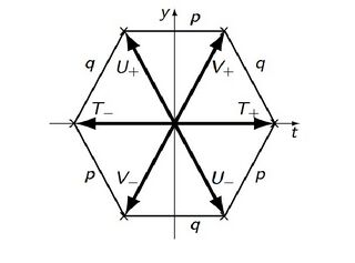
The representation of generators of the SU(3) group.
.jpeg)
Here,
and
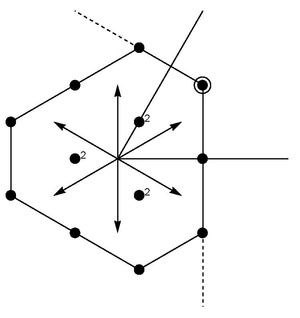
All the other states of the representation can be constructed by the successive application of the ladder operators and and by identifying the base states which are annihilated by the action of the lowering operators. These operators can be pictured as arrows whose endpoints form the vertices of a hexagon (picture for generators above).
Clebsch–Gordan coefficient for SU(3)
The product representation of two irreducible representations and is generally reducible. Symbolically,
where is an integer.
For example, two octets (adjoints) compose to
that is, their product reduces to an icosaseptet (27), decuplet, two octets, an antidecuplet, and a singlet, 64 states in all.
The right-hand series is called the Clebsch–Gordan series. It implies that the representation appears times in the reduction of this direct product of with .
Now a complete set of operators is needed to specify uniquely the states of each irreducible representation inside the one just reduced. The complete set of commuting operators in the case of the irreducible representation is
where
- .
The states of the above direct product representation are thus completely represented by the set of operators
where the number in the parentheses designates the representation on which the operator acts.
An alternate set of commuting operators can be found for the direct product representation, if one considers the following set of operators,[15]
Thus, the set of commuting operators includes
This is a set of nine operators only. But the set must contain ten operators to define all the states of the direct product representation uniquely. To find the last operator Γ, one must look outside the group. It is necessary to distinguish different for similar values of P and Q.
Thus, any state in the direct product representation can be represented by the ket,
also using the second complete set of commuting operator, we can define the states in the direct product representation as
We can drop the from the state and label the states as
using the operators from the first set, and,
using the operators from the second set.
Both these states span the direct product representation and any states in the representation can be labeled by suitable choice of the eigenvalues.
Using the completeness relation,
Here, the coefficients
are the Clebsch–Gordan coefficients.
A different notation
To avoid confusion, the eigenvalues can be simultaneously denoted by μ and the eigenvalues are simultaneously denoted by ν. Then the eigenstate of the direct product representation can be denoted by[15]
where is the eigenvalues of and is the eigenvalues of denoted simultaneously. Here, the quantity expressed by the parenthesis is the Wigner 3-j symbol.
Furthermore, are considered to be the basis states of and are the basis states of . Also are the basis states of the product representation. Here represents the combined eigenvalues and respectively.
Thus the unitary transformations that connects the two bases are
This is a comparatively compact notation. Here,
are the Clebsch–Gordan coefficients.
Orthogonality relations
The Clebsch–Gordan coefficients form a real orthogonal matrix. Therefore,
Also, they follow the following orthogonality relations,
Symmetry properties
If an irreducible representation appears in the Clebsch–Gordan series of , then it must appear in the Clebsch–Gordan series of . Which implies,
Where
Since the Clebsch–Gordan coefficients are all real, the following symmetry property can be deduced,
Where .
Symmetry group of the 3D oscillator Hamiltonian operator
A three-dimensional harmonic oscillator is described by the Hamiltonian
where the spring constant, the mass and Planck's constant have been absorbed into the definition of the variables, ħ=m=1.
It is seen that this Hamiltonian is symmetric under coordinate transformations that preserve the value of . Thus, any operators in the group SO(3) keep this Hamiltonian invariant.
More significantly, since the Hamiltonian is Hermitian, it further remains invariant under operation by elements of the much larger SU(3) group.
A symmetric (dyadic) tensor operator analogous to the Laplace–Runge–Lenz vector for the Kepler problem may be defined,
which commutes with the Hamiltonian,
Since it commutes with the Hamiltonian (its trace), it represents 6−1=5 constants of motion.
It has the following properties,
Apart from the tensorial trace of the operator, which is the Hamiltonian, the remaining 5 operators can be rearranged into their spherical component form as
Further, the angular momentum operators are written in spherical component form as
They obey the following commutation relations,
The eight operators (consisting of the 5 operators derived from the traceless symmetric tensor operator Âij and the three independent components of the angular momentum vector) obey the same commutation relations as the infinitesimal generators of the SU(3) group, detailed above.
As such, the symmetry group of Hamiltonian for a linear isotropic 3D Harmonic oscillator is isomorphic to SU(3) group.
More systematically, operators such as the Ladder operators
- and
can be constructed which raise and lower the eigenvalue of the Hamiltonian operator by 1.
The operators âi and âi† are not hermitian; but hermitian operators can be constructed from different combinations of them,
- namely, .
There are nine such operators for i,j=1,2,3.
The nine hermitian operators formed by the bilinear forms âi†âj are controlled by the fundamental commutators
and seen to not commute among themselves. As a result, this complete set of operators don't share their eigenvectors in common, and they cannot be diagonalized simultaneously. The group is thus non-Abelian and degeneracies may be present in the Hamiltonian, as indicated.
The Hamiltonian of the 3D isotropic harmonic oscillator, when written in terms of the operator amounts to
- .
The Hamiltonian has 8-fold degeneracy. A successive application of âi and âj† on the left preserves the Hamiltonian invariant, since it increases Ni by 1 and decrease Nj by 1, thereby keeping the total
- constant. (cf. quantum harmonic oscillator)
The maximally commuting set of operators
Since the operators belonging to the symmetry group of Hamiltonian do not always form an Abelian group, a common eigenbasis cannot be found that diagonalizes all of them simultaneously. Instead, we take the maximally commuting set of operators from the symmetry group of the Hamiltonian, and try to reduce the matrix representations of the group into irreducible representations.
Hilbert space of two systems
The Hilbert space of two particles is the tensor product of the two Hilbert spaces of the two individual particles,
where and are the Hilbert space of the first and second particles, respectively.
The operators in each of the Hilbert spaces have their own commutation relations, and an operator of one Hilbert space commutes with an operator from the other Hilbert space. Thus the symmetry group of the two particle Hamiltonian operator is the superset of the symmetry groups of the Hamiltonian operators of individual particles. If the individual Hilbert spaces are N dimensional, the combined Hilbert space is N2 dimensional.
Clebsch–Gordan coefficient in this case
The symmetry group of the Hamiltonian is SU(3). As a result, the Clebsch–Gordan coefficients can be found by expanding the uncoupled basis vectors of the symmetry group of the Hamiltonian into its coupled basis. The Clebsch–Gordan series is obtained by block-diagonalizing the Hamiltonian through the unitary transformation constructed from the eigenstates which diagonalizes the maximal set of commuting operators.
Young tableaux
A Young tableau (plural tableaux) is a method for decomposing products of an SU(N) group representation into a sum of irreducible representations. It provides the dimension and symmetry types of the irreducible representations, which is known as the Clebsch–Gordan series. Each irreducible representation corresponds to a single-particle state and a product of more than one irreducible representation indicates a multiparticle state.
Since the particles are mostly indistinguishable in quantum mechanics, this approximately relates to several permutable particles. The permutations of n identical particles constitute the symmetric group Sn. Every n-particle state of Sn that is made up of single-particle states of the fundamental N-dimensional SU(N) multiplet belongs to an irreducible SU(N) representation. Thus, it can be used to determine the Clebsch–Gordan series for any unitary group.[17]
Constructing the states
Any two particle wavefunction , where the indices 1,2 represents the state of particle 1 and 2, can be used to generate states of explicit symmetry using the symmetrizing and the anti-symmetrizing operators.[18]
where the are the operator that interchanges the particles (Exchange operator).
The following relation follows:[18]-
thus,
Starting from a multiparticle state, we can apply and repeatedly to construct states that are:[18]
- Symmetric with respect to all particles.
- Antisymmetric with respect to all particles.
- Mixed symmetries, i.e. symmetric or antisymmetric with respect to some particles.
Constructing the tableaux
Instead of using ψ, in Young tableaux, we use square boxes (□) to denote particles and i to denote the state of the particles.

The complete set of particles are denoted by arrangements of □s, each with its own quantum number label (i).
The tableaux is formed by stacking boxes side by side and up-down such that the states symmetrised with respect to all particles are given in a row and the states anti-symmetrised with respect to all particles lies in a single column. Following rules are followed while constructing the tableaux:[17]
- A row must not be longer than the one before it.
- The quantum labels (numbers in the □) should not decrease while going left to right in a row.
- The quantum labels must strictly increase while going down in a column.
Case for N = 3
For N=3 that is in the case of SU(3), the following situation arises. In SU(3) there are three labels, they are generally designated by (u,d,s) corresponding to up, down and strange quarks which follows the SU(3) algebra. They can also be designated generically as (1,2,3). For a two-particle system, we have the following six symmetry states:
and the following three antisymmetric states:
The 1-column, 3-row tableau is the singlet, and so all tableaux of nontrivial irreps of SU(3) cannot have more than two rows. The representation D(p,q) has p+q boxes on the top row and q boxes on the second row.
Clebsch–Gordan series from the tableaux
Clebsch–Gordan series is the expansion of the tensor product of two irreducible representation into direct sum of irreducible representations. . This can be easily found out from the Young tableaux.
Procedure to obtain the Clebsch–Gordan series from Young tableaux: The following steps are followed to construct the Clebsch–Gordan series from the Young tableaux:[19]
- Write down the two Young diagrams for the two irreps under consideration, such as in the following example. In the second figure insert a series of the letter a in the first row, the letter b in the second row, the letter c in the third row, etc. in order to keep track of them once they are included in the various resultant diagrams:
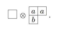
- Take the first box containing an a and appends it to the first Young diagram in all possible ways that follow the rules for creation of a Young diagram:
- Then take the next box containing an a and do the same thing with it, except that we are not allowed to put two a's together in the same column.
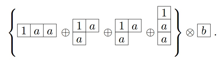
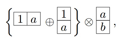
The last diagram in the curly bracket contains two a in the same column thus the diagram must be deleted. Thereby giving:
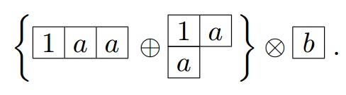
- Append the last box to the diagram in curly bracket in all possible ways resulting in:
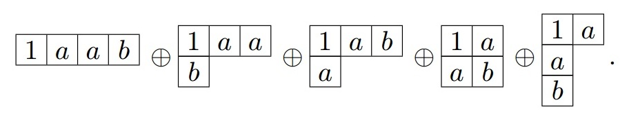
- In each rows while counting from right to left, if at any point the number of a particular alphabet encountered be more than the number of the previous alphabet, then the diagram must be deleted. Here the first and the third diagram should be deleted, resulting in:


Example of Clebsch–Gordan series for SU(3)
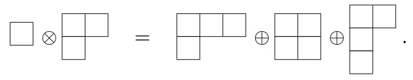
The tensor product of a triplet with an octet reducing to a deciquintuplet (15), an anti-sextet, and a triplet
appears diagrammatically as[19]-


a total of 24 states. Using the same procedure, any direct product representation is easily reduced.
See also
- Wigner D-matrix
- Tensor operator
- Wigner-Eckart theorem
- Representation theory
- Racah W-coefficient
- Gell-Mann–Okubo mass formula
References
- ↑ P. Carruthers (1966) Introduction to Unitary symmetry, Interscience. online.
- ↑ Introduction to Elementary Particles- David J. Griffiths, ISBN 978-3527406012, Chapter-1, Page33-38
- ↑ Hall 2015 Section 6.2
- ↑ Bargmann, V.; Moshinsky, M. (1961). "Group theory of harmonic oscillators (II). The integrals of Motion for the quadrupole-quadrupole interaction". Nuclear Physics 23: 177–199. doi:10.1016/0029-5582(61)90253-X. Bibcode: 1961NucPh..23..177B.
- ↑ See eq. 3.65 in Pais, A. (1966). "Dynamical Symmetry in Particle Physics". Reviews of Modern Physics 38 (2): 215–255. doi:10.1103/RevModPhys.38.215. Bibcode: 1966RvMP...38..215P.
- ↑ Pais, ibid. (3.66)
- ↑ Hall 2015 Chapter 6
- ↑ Hall 2015 Proposition 13.11
- ↑ Hall 2015 Theorem 5.6
- ↑ Hall 2015 Section 3.6
- ↑ See the proof of Proposition 6.17 in Hall 2015
- ↑ Hall 2015 Theorem 6.27 and Example 10.23
- ↑ 13.0 13.1 Greiner & Müller 2012, Ch. 10.15 Note: There is a typo in the final quoting of the result - in Equation 10.121 the first should instead be a .
- ↑ Senner & Schulten
- ↑ 15.0 15.1 De Swart, J. J. (1963). "The Octet Model and its Clebsch-Gordan Coefficients". Reviews of Modern Physics 35 (4): 916–939. doi:10.1103/RevModPhys.35.916. Bibcode: 1963RvMP...35..916D. https://cds.cern.ch/record/345262/files/RevModPhys.35.916.pdf. (Erratum: [De Swart, J. J. (1965). "none". Reviews of Modern Physics 37 (2): 326. doi:10.1103/RevModPhys.37.326. Bibcode: 1965RvMP...37..326D.])
- ↑ Fradkin, D. M. (1965). "Three-Dimensional Isotropic Harmonic Oscillator and SU3". American Journal of Physics 33 (3): 207–211. doi:10.1119/1.1971373. Bibcode: 1965AmJPh..33..207F.
- ↑ 17.0 17.1 Arfken, George B.; Weber, Hans J. (2005). "4. Group Theory". Mathematical Methods For Physicists International Student Edition (6th ed.). Elsevier. pp. 241–320. ISBN 978-0-08-047069-6. https://books.google.com/books?id=tNtijk2iBSMC&pg=PA241.
- ↑ 18.0 18.1 18.2 http://hepwww.rl.ac.uk/Haywood/Group_Theory_Lectures/Lecture_4.pdf [bare URL PDF]
- ↑ 19.0 19.1 "Some Notes on Young Tableaux as useful for irreps for su(n)". http://physics.unm.edu/Courses/Finley/p467/handouts/YoungTableauxSubs.pdf.
- Lichtenberg, D.B. (2012). Unitary Symmetry and Elementary Particles (2nd ed.). Academic Press. ISBN 978-0123941992.
- Greiner, W.; Müller, B. (2012). Quantum Mechanics: Symmetries (2nd ed.). Springer. ISBN 978-3540580805. https://archive.org/details/quantummechanics0001grei.
- Hall, Brian C. (2015), Lie Groups, Lie Algebras, and Representations: An Elementary Introduction, Graduate Texts in Mathematics, 222 (2nd ed.), Springer, ISBN 978-3319134666
- McNamee, P.; j., S.; Chilton, F. (1964). "Tables of Clebsch-Gordan Coefficients of SU3". Reviews of Modern Physics 36 (4): 1005. doi:10.1103/RevModPhys.36.1005. Bibcode: 1964RvMP...36.1005M.
- Mandel'tsveig, V. B. (1965). "Irreducible representations of the SU3 group". Sov Phys JETP 20 (5): 1237–1243. online
- Coleman, Sidney (1965). "Fun with SU(3)". IAEA. https://inspirehep.net/literature/1720680.
- Pluhar, Z.; Smirnov, Yu F.; Tolstoy, V. N. (1986). "Clebsch-Gordan coefficients of SU(3) with simple symmetry properties". Journal of Physics A: Mathematical and General 19 (1): 21–28. doi:10.1088/0305-4470/19/1/007. Bibcode: 1986JPhA...19...21P.
 |  |

