Physics:Curie's law
For many paramagnetic materials, the magnetization of the material is directly proportional to an applied magnetic field, for sufficiently high temperatures and small fields. However, if the material is heated, this proportionality is reduced. For a fixed value of the field, the magnetic susceptibility is inversely proportional to temperature, that is
where
- is the (volume) magnetic susceptibility,
- is the magnitude of the resulting magnetization (A/m),
- is the magnitude of the applied magnetic field (A/m),
- is absolute temperature (K),
- is a material-specific Curie constant (K).
Pierre Curie discovered this relation, now known as Curie's law, by fitting data from experiment. It only holds for high temperatures and weak magnetic fields. As the derivations below show, the magnetization saturates in the opposite limit of low temperatures and strong fields. If the Curie constant is null, other magnetic effects dominate, like Langevin diamagnetism or Van Vleck paramagnetism.
Derivation with quantum mechanics

A simple model of a paramagnet concentrates on the particles which compose it which do not interact with each other. Each particle has a magnetic moment given by . The energy of a magnetic moment in a magnetic field is given by
where is the magnetic field density, measured in teslas (T).
Two-state (spin-½) particles
To simplify the calculation, we are going to work with a 2-state particle: it may either align its magnetic moment with the magnetic field or against it. So the only possible values of magnetic moment are then and . If so, then such a particle has only two possible energies, when it is aligned with the field and when it is oriented opposite to the field.
The extent to which the magnetic moments are aligned with the field can be calculated from the partition function. For a single particle, this is
The partition function for a set of N such particles, if they do not interact with each other, is
and the free energy is therefore
The magnetization is the negative derivative of the free energy with respect to the applied field, and so the magnetization per unit volume is
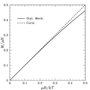
where n is the number density of magnetic moments.[1]: 117 The formula above is known as the Langevin paramagnetic equation. Pierre Curie found an approximation to this law that applies to the relatively high temperatures and low magnetic fields used in his experiments. As temperature increases and magnetic field decreases, the argument of the hyperbolic tangent decreases. In the Curie regime,
Moreover, if , then
so the magnetization is small, and we can write , and thus
In this regime, the magnetic susceptibility given by
yields
with a Curie constant given by , in kelvins (K).[2]
In the regime of low temperatures or high fields, tends to a maximum value of , corresponding to all the particles being completely aligned with the field. Since this calculation doesn't describe the electrons embedded deep within the Fermi surface, forbidden by the Pauli exclusion principle to flip their spins, it does not exemplify the quantum statistics of the problem at low temperatures. Using the Fermi–Dirac distribution, one will find that at low temperatures is linearly dependent on the magnetic field, so that the magnetic susceptibility saturates to a constant.
General case
When the particles have an arbitrary spin (any number of spin states), the formula is a bit more complicated. At low magnetic fields or high temperature, the spin follows Curie's law, with[3]
where is the total angular momentum quantum number, and is the spin's g-factor (such that is the magnetic moment). For a two-level system with magnetic moment , the formula reduces to as above, while the corresponding expressions in Gaussian units are
For this more general formula and its derivation (including high field, low temperature) see the article Brillouin function. As the spin approaches infinity, the formula for the magnetization approaches the classical value derived in the following section.
Derivation with classical statistical mechanics
An alternative treatment applies when the paramagnets are imagined to be classical, freely-rotating magnetic moments. In this case, their position will be determined by their angles in spherical coordinates, and the energy for one of them will be:
where is the angle between the magnetic moment and the magnetic field (which we take to be pointing in the coordinate.) The corresponding partition function is
We see there is no dependence on the angle, and also we can change variables to to obtain
Now, the expected value of the component of the magnetization (the other two are seen to be null (due to integration over ), as they should) will be given by
To simplify the calculation, we see this can be written as a differentiation of :
(This approach can also be used for the model above, but the calculation was so simple this is not so helpful.)
Carrying out the derivation we find
where is the Langevin function:
This function would appear to be singular for small , but it is not, since the two singular terms cancel each other. In fact, its behavior for small arguments is , so the Curie limit also applies, but with a Curie constant three times smaller in this case. Similarly, the function saturates at for large values of its argument, and the opposite limit is likewise recovered.
History
Pierre Curie observed in 1895 that the magnetic susceptibility of oxygen is inversely proportional to temperature. Paul Langevin presented a classical derivation of this relationship ten years later.[4]
See also
References
- ↑ Kardar, Mehran (2007). Statistical Physics of Particles. Cambridge University Press. ISBN 978-0-521-87342-0. OCLC 860391091.
- ↑ Coey, J. M. D.; Coey, J. M. D. (2010-03-25) (in en). Magnetism and Magnetic Materials. Cambridge University Press. ISBN 978-0-521-81614-4. https://books.google.com/books?id=Ie72CFd-eSEC.
- ↑ Kittel, Charles (11 November 2004). Introduction to Solid State Physics (8th ed.). Wiley. pp. 304. ISBN 0-471-41526-X.
- ↑ Van Vleck, J. H. (1978-07-14). "Quantum Mechanics: The Key to Understanding Magnetism". Science 201 (4351): 113–120. doi:10.1126/science.201.4351.113.
External links
- Curie's law at Merriam-Webster
 |
