Physics:Frank-Kamenetskii theory

Short description: Scientific theory that explains thermal explosions

In combustion, Frank-Kamenetskii theory explains the thermal explosion of a homogeneous mixture of reactants, kept inside a closed vessel with constant temperature walls. It is named after a Russian scientist David A. Frank-Kamenetskii, who along with Nikolay Semenov developed the theory in the 1930s.

Problem description

Sources:

Consider a vessel maintained at a constant temperature [math]\displaystyle{ T_o }[/math], containing a homogeneous reacting mixture. Let the characteristic size of the vessel be [math]\displaystyle{ a }[/math]. Since the mixture is homogeneous, the density [math]\displaystyle{ \rho }[/math] is constant. During the initial period of ignition, the consumption of reactant concentration is negligible (see [math]\displaystyle{ t_f }[/math] and [math]\displaystyle{ t_e }[/math] below), thus the explosion is governed only by the energy equation. Assuming a one-step global reaction [math]\displaystyle{ \text{fuel} + \text{oxidizer} \rightarrow \text{products} + q }[/math], where [math]\displaystyle{ q }[/math] is the amount of heat released per unit mass of fuel consumed, and a reaction rate governed by Arrhenius law, the energy equation becomes

[math]\displaystyle{ \rho c_v \frac{\partial T}{\partial t} = \lambda \nabla^2 T + q \rho B Y_{Fo} e^{-E/(RT)} }[/math]

where

[math]\displaystyle{ T }[/math]	is the temperature of the mixture;
[math]\displaystyle{ c_v }[/math]	is the specific heat at constant volume;
[math]\displaystyle{ \lambda }[/math]	is the thermal conductivity;
[math]\displaystyle{ B }[/math]	is the pre-exponential factor with dimension of one over time;
[math]\displaystyle{ Y_{Fo} }[/math]	is the initial fuel mass fraction;
[math]\displaystyle{ E }[/math]	is the activation energy;
[math]\displaystyle{ R }[/math]	is the universal gas constant.

Non-dimensionalization

Non-dimensional scales of time, temperature, length, and heat transfer may be defined as

[math]\displaystyle{ \tau = \frac{t}{t_e}, \quad \theta = \frac{\beta(T-T_o)}{T_o}, \quad \eta^j = \frac{r^j} a, \quad \delta = \frac{t_c}{t_e} }[/math]

where

[math]\displaystyle{ t_c = \rho c_va^2/ \lambda }[/math]	is the characteristic heat conduction time across the vessel;
[math]\displaystyle{ t_f = \left(B e^{-\beta}\right)^{\!-1} }[/math]	is the characteristic fuel consumption time;
[math]\displaystyle{ t_e = \left(\beta\gamma B e^{-\beta}\right)^{\!-1} }[/math]	is the characteristic explosion/ignition time;
[math]\displaystyle{ a }[/math]	is the characteristic distance, e.g., vessel radius;
[math]\displaystyle{ \beta = E/(R\,T_o) }[/math]	is the non-dimensional activation energy;
[math]\displaystyle{ \gamma = (q Y_{Fo})/(c_v T_o) }[/math]	is the heat-release parameter;
[math]\displaystyle{ \delta }[/math]	is the Damköhler number;
[math]\displaystyle{ r }[/math]	is the spatial coordinate with origin at the center;
[math]\displaystyle{ j=0 }[/math]	for planar slab;
[math]\displaystyle{ j=1 }[/math]	for cylindrical vessel;
[math]\displaystyle{ j=2 }[/math]	for spherical vessel.

Note

In a typical combustion process, [math]\displaystyle{ \gamma\approx 6{-}8,\ \beta\approx 30{-}100 }[/math] so that [math]\displaystyle{ \beta\gamma\gg 1 }[/math].

Therefore, [math]\displaystyle{ t_f = \beta\gamma t_e \gg 1 }[/math]. That is, fuel consumption time is much longer than ignition time, so fuel consumption is essentially negligible in the study of ignition.

This is why the fuel concentration is assumed to remain the initial fuel concentration [math]\displaystyle{ Y_{Fo} }[/math].

Substituting the non-dimensional variables in the energy equation from the introduction

[math]\displaystyle{ \frac{\partial\theta}{\partial \tau} = \frac 1 {\delta}\frac 1 {\eta^j} \frac{\partial}{\partial \eta} \left(\eta^j \frac{\partial \theta}{\partial \eta}\right) + e^{\theta/(1+\theta/\beta)} }[/math]

Since [math]\displaystyle{ \beta\gg 1 }[/math], the exponential term can be linearized [math]\displaystyle{ e^{\theta/(1+\theta/\beta)}\approx e^\theta }[/math], hence

[math]\displaystyle{ \frac{\partial\theta}{\partial \tau} = \frac 1 \delta \frac 1 {\eta^j} \frac \partial {\partial \eta} \left(\eta^j \frac{\partial \theta}{\partial \eta}\right) + e^\theta }[/math]

At [math]\displaystyle{ \tau=0 }[/math], we have [math]\displaystyle{ \theta(\eta,0)=0 }[/math] and for [math]\displaystyle{ \tau\gt 0 }[/math], [math]\displaystyle{ \theta }[/math] needs to satisfy [math]\displaystyle{ \theta(1,\tau)=0 }[/math] and [math]\displaystyle{ \partial\theta/\partial \eta |_{\eta=0} = 0. }[/math]

Semenov theory

Solution of Semenov problem

Before Frank-Kamenetskii, his doctoral advisor Nikolay Semyonov (or Semenov) proposed a thermal explosion theory with a simpler model with which he assumed a linear function for the heat conduction process instead of the Laplacian operator. Semenov's equation reads as

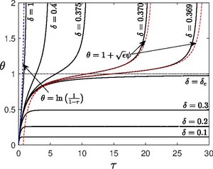
[math]\displaystyle{ \frac{d\theta}{d\tau} = e^\theta - \frac{\theta}{\delta}, \quad \theta(0)=0 }[/math]

in which the exponential term [math]\displaystyle{ e^\theta }[/math] will tend to increase [math]\displaystyle{ \theta }[/math] as time proceeds whereas the linear term [math]\displaystyle{ -\theta/\delta }[/math] will tend to decrease [math]\displaystyle{ \theta }[/math]. The relevant importance between the two terms are determined by the Damköhler number [math]\displaystyle{ \delta }[/math]. The numerical solution of the above equation for different values of [math]\displaystyle{ \delta }[/math] is shown in the figure.

Steady-state regime

When [math]\displaystyle{ 0\lt \delta\lt e^{-1} }[/math], the linear term eventually dominates and the system is able to reach a steady state as [math]\displaystyle{ \tau\rightarrow \infty }[/math]. At steady state ([math]\displaystyle{ d\theta/d\tau=0 }[/math]), the balance is given by the equation

[math]\displaystyle{ \delta e^\theta= \theta, \quad \Rightarrow \quad \theta = -W(-\delta) }[/math]

where [math]\displaystyle{ W }[/math] represents the Lambert W function. From the properties of Lambert W function, it is easy to see that the steady state temperature provided by the above equation exists only when [math]\displaystyle{ \delta\leq \delta_c=1/e }[/math], where [math]\displaystyle{ \delta_c }[/math] is called as Frank-Kamenetskii parameter as a critical point where the system bifurcates from the existence of steady state to explosive state at large times.

Explosive regime

For [math]\displaystyle{ \delta_c\lt \delta\lt \infty }[/math], the system explodes since the exponential term dominates as time proceeds. We do not need to wait for a long time for [math]\displaystyle{ \theta }[/math] to blow up. Because of the exponential forcing, [math]\displaystyle{ \theta\rightarrow\infty }[/math] at a finite value of [math]\displaystyle{ \tau }[/math]. This time is interpreted as the ignition time or induction time of the system. When [math]\displaystyle{ \delta\gg \delta_c }[/math], the heat conduction term [math]\displaystyle{ -\theta/\delta }[/math] can be neglected in which case the problem admits an explicit solution,

[math]\displaystyle{ \frac{d\theta}{d \tau} = e^\theta, \quad \Rightarrow \quad \theta = \ln \left(\frac 1 {1-\tau}\right) }[/math]

At time [math]\displaystyle{ \tau=1 }[/math], the system explodes. This time is also referred to as the adiabatic induction period since the heat conduction term [math]\displaystyle{ -\theta/\delta }[/math] is neglected.

In the near-critical condition, i.e., when [math]\displaystyle{ \delta-\delta_c\rightarrow 0^+ }[/math], the system takes very long time to explode. The analysis for this limit was first carried out by Frank-Kamenetskii., although proper asymptotics were carried out only later by D. R. Kassoy and Amable Liñán including reactant consumption because reactant consumption is not negligible when [math]\displaystyle{ \tau\sim \beta\gamma }[/math]. A simplified analysis without reactant consumption is presented here. Let us define a small parameter [math]\displaystyle{ \epsilon\rightarrow 0^+ }[/math] such that [math]\displaystyle{ \delta=\delta_c(1+\epsilon) }[/math]. For this case, the time evolution of [math]\displaystyle{ \theta }[/math] is as follows: first it increases to steady-state temperature value corresponding to [math]\displaystyle{ \delta=\delta_c }[/math], which is given by [math]\displaystyle{ \theta=-W(-\delta_c)=1 }[/math] at times of order [math]\displaystyle{ \tau\sim O(1) }[/math], then it stays very close to this steady-state value for a long time before eventually exploding at a long time. The quantity of interest is the long-time estimate for the explosion. To find out the estimate, introduce the transformations [math]\displaystyle{ \zeta=\sqrt{\epsilon}\tau }[/math] and [math]\displaystyle{ \theta=1+\sqrt{\epsilon}\psi(\zeta) -\epsilon }[/math] that is appropriate for the region where [math]\displaystyle{ \theta }[/math] stays close to [math]\displaystyle{ 1 }[/math] into the governing equation and collect only the leading-order terms to find out

[math]\displaystyle{ \delta_c\frac{d\psi}{d\zeta} = 1+\frac{\psi^2}{2}, \quad \psi(0)\rightarrow -(1-\theta)/\sqrt{\epsilon}=-\infty }[/math]

where the boundary condition is derived by matching with the initial region wherein [math]\displaystyle{ \tau,\theta\sim 1 }[/math]. The solution to the above-mentioned problem is given by

[math]\displaystyle{ \psi= - \sqrt{2}\cot\left(\frac{\zeta}{\sqrt 2\delta_c}\right) }[/math]

which immediately reveals that [math]\displaystyle{ \psi\rightarrow \infty }[/math] when [math]\displaystyle{ \zeta= \sqrt 2 \pi \delta_c. }[/math] Writing this condition in terms of [math]\displaystyle{ \tau }[/math], the explosion time in the near-critical condition is found to be

[math]\displaystyle{ \tau = \sqrt{\frac{2\pi^2\delta_c^3}{\delta-\delta_c}} }[/math]

which implies that the ignition time [math]\displaystyle{ \tau\rightarrow \infty }[/math] as [math]\displaystyle{ \delta-\delta_c\rightarrow 0^+ }[/math] with a square-root singularity.

Frank-Kamenetskii steady-state theory

The only parameter which characterizes the explosion is the Damköhler number [math]\displaystyle{ \delta }[/math]. When [math]\displaystyle{ \delta }[/math] is very high, conduction time is longer than the chemical reaction time and the system explodes with high temperature since there is not enough time for conduction to remove the heat. On the other hand, when [math]\displaystyle{ \delta }[/math] is very low, heat conduction time is much faster than the chemical reaction time, such that all the heat produced by the chemical reaction is immediately conducted to the wall, thus there is no explosion, it goes to an almost steady state, Amable Liñán coined this mode as slowly reacting mode. At a critical Damköhler number [math]\displaystyle{ \delta_c }[/math] the system goes from slowly reacting mode to explosive mode. Therefore, [math]\displaystyle{ \delta\lt \delta_c }[/math], the system is in steady state. Instead of solving the full problem to find this [math]\displaystyle{ \delta_c }[/math], Frank-Kamenetskii solved the steady state problem for various Damköhler number until the critical value, beyond which no steady solution exists. So the problem to be solved is

[math]\displaystyle{ \frac 1 {\eta^j} \frac d {d \eta} \left(\eta^j \frac{d \theta}{d \eta}\right) = - \delta e^\theta }[/math]

with boundary conditions

[math]\displaystyle{ \theta(1)=0, \quad \frac{d\theta}{d\eta}_{\eta=0}=0 }[/math]

the second condition is due to the symmetry of the vessel. The above equation is special case of Liouville–Bratu–Gelfand equation in mathematics.

Planar vessel

Frank-Kamenetskii explosion for planar vessel

For planar vessel, there is an exact solution. Here [math]\displaystyle{ j=0 }[/math], then

[math]\displaystyle{ \frac{d^2\theta}{d\eta^2} = -\delta e^\theta }[/math]

If the transformations [math]\displaystyle{ \Theta= \theta_m-\theta }[/math] and [math]\displaystyle{ \xi^2 = \delta e^{\theta_m} \eta^2 }[/math], where [math]\displaystyle{ \theta_m }[/math] is the maximum temperature which occurs at [math]\displaystyle{ \eta=0 }[/math] due to symmetry, are introduced

[math]\displaystyle{ \frac{d^2\Theta}{d\xi^2} = e^{-\Theta}, \quad \Theta(0)=0, \quad \frac{d\Theta}{d\xi}_{\xi=0}=0 }[/math]

Integrating once and using the second boundary condition, the equation becomes

[math]\displaystyle{ \frac{d\Theta}{d\xi} = \sqrt{2(1-e^{-\Theta})} }[/math]

and integrating again

[math]\displaystyle{ e^{(\theta_m-\theta)/2} = \cosh \left(\eta \sqrt{\frac{\delta e^{\theta_m}}{2}} \right) }[/math]

The above equation is the exact solution, but [math]\displaystyle{ \theta_m }[/math] maximum temperature is unknown, but we have not used the boundary condition of the wall yet. Thus using the wall boundary condition [math]\displaystyle{ \theta=0 }[/math] at [math]\displaystyle{ \eta=1 }[/math], the maximum temperature is obtained from an implicit expression,

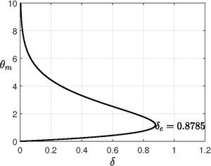
[math]\displaystyle{ e^{\theta_m/2} = \cosh \sqrt{\frac{\delta e^{\theta_m}} 2} \quad \text{or} \quad \delta = 2 e^{-\theta_m} \left(\operatorname{arcosh} e^{\theta_m/2}\right)^{\!2} }[/math]

Critical [math]\displaystyle{ \delta_c }[/math] is obtained by finding the maximum point of the equation (see figure), i.e., [math]\displaystyle{ d\delta/d\theta_m=0 }[/math] at [math]\displaystyle{ \delta_c }[/math].

[math]\displaystyle{ \frac{d\delta}{d\theta_m}=0, \quad \Rightarrow \quad e^{\theta_{m,c}/2} - \sqrt{e^{\theta_{m,c}}-1}\operatorname{arcosh} e^{\theta_{m,c}/2} =0 }[/math]

[math]\displaystyle{ \theta_{m,c}= 1.1868, \quad \Rightarrow \quad \delta_c = 0.8785 }[/math]

So the critical Frank-Kamentskii parameter is [math]\displaystyle{ \delta_c=0.8785 }[/math]. The system has no steady state (or explodes) for [math]\displaystyle{ \delta\gt \delta_c=0.8785 }[/math] and for [math]\displaystyle{ \delta\lt \delta_c=0.8785 }[/math], the system goes to a steady state with very slow reaction.

Cylindrical vessel

Frank-Kamenetskii explosion for cylindrical vessel

For cylindrical vessel, there is an exact solution. Though Frank-Kamentskii used numerical integration assuming there is no explicit solution, Paul L. Chambré provided an exact solution in 1952. H. Lemke also solved provided a solution in a somewhat different form in 1913. Here [math]\displaystyle{ j=1 }[/math], then

[math]\displaystyle{ \frac 1 \eta \frac d {d\eta}\left(\eta\frac{d\theta}{d\eta}\right) = -\delta e^\theta }[/math]

If the transformations [math]\displaystyle{ \omega= \eta d\theta/d\eta }[/math] and [math]\displaystyle{ \chi = e^{\theta} \eta^2 }[/math] are introduced

[math]\displaystyle{ \frac{d\omega}{d\chi} = -\frac{\delta}{2+\omega}, \quad \omega(0)=0 }[/math]

The general solution is [math]\displaystyle{ \omega^2 + 4\omega + C = -2\delta\chi }[/math]. But [math]\displaystyle{ C=0 }[/math] from the symmetry condition at the centre. Writing back in original variable, the equation reads,

[math]\displaystyle{ \eta^2 \left(\frac{d\theta}{d\eta}\right)^2+ 4\eta \frac{d\theta}{d\eta} = - 2\delta\eta^2 e^\theta }[/math]

But the original equation multiplied by [math]\displaystyle{ 2\eta^2 }[/math] is

[math]\displaystyle{ 2\eta^2 \frac{d^2\theta}{d\eta^2} + 2\eta \frac{d\theta}{d\eta} = -2 \delta \eta^2 e^\theta }[/math]

Now subtracting the last two equation from one another leads to

[math]\displaystyle{ \frac{d^2\theta}{d\eta^2} - \frac{1}{\eta} \frac{d\theta}{d\eta} - \frac{1}{2} \left(\frac{d\theta}{d\eta}\right)^2 =0 }[/math]

This equation is easy to solve because it involves only the derivatives, so letting [math]\displaystyle{ g(\eta)=d\theta/d\eta }[/math] transforms the equation

[math]\displaystyle{ \frac{dg}{d\eta} - \frac{g}{\eta} - \frac{g^2}{2}=0 }[/math]

This is a Bernoulli differential equation of order [math]\displaystyle{ 2 }[/math], a type of Riccati equation. The solution is

[math]\displaystyle{ g(\eta) = \frac{d\theta}{d\eta} = -\frac{4\eta}{B'+\eta^2} }[/math]

Integrating once again, we have [math]\displaystyle{ \theta = A - 2\ln ( B\eta^2 + 1) }[/math] where [math]\displaystyle{ B = 1/B' }[/math]. We have used already one boundary condition, there is one more boundary condition left, but with two constants [math]\displaystyle{ A, \ B }[/math]. It turns out [math]\displaystyle{ A }[/math] and [math]\displaystyle{ B }[/math] are related to each other, which is obtained by substituting the above solution into the starting equation we arrive at [math]\displaystyle{ A = \ln (8B/\delta) }[/math]. Therefore, the solution is

[math]\displaystyle{ \theta = \ln \frac{8B/\delta}{(B\eta^2+1)^2} }[/math]

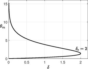
Now if we use the other boundary condition [math]\displaystyle{ \theta(1)=0 }[/math], we get an equation for [math]\displaystyle{ B }[/math] as [math]\displaystyle{ \delta(B+1)^2 - 8B =0 }[/math]. The maximum value of [math]\displaystyle{ \delta }[/math] for which solution is possible is when [math]\displaystyle{ B=1 }[/math], so the critical Frank-Kamentskii parameter is [math]\displaystyle{ \delta_c=2 }[/math]. The system has no steady state( or explodes) for [math]\displaystyle{ \delta\gt \delta_c=2 }[/math] and for [math]\displaystyle{ \delta\lt \delta_c=2 }[/math], the system goes to a steady state with very slow reaction. The maximum temperature [math]\displaystyle{ \theta_m }[/math] occurs at [math]\displaystyle{ \eta=0 }[/math]

[math]\displaystyle{ \theta_m= \ln \frac{8B}{\delta} \quad \text{or} \quad \delta= 8B e^{-\theta_m} }[/math]

For each value of [math]\displaystyle{ \delta }[/math], we have two values of [math]\displaystyle{ \theta_m }[/math] since [math]\displaystyle{ B }[/math] is multi-valued. The maximum critical temperature is [math]\displaystyle{ \theta_{m,c} = \ln 4 }[/math].

Spherical vessel

Frank-Kamenetskii spherical vessel

For spherical vessel, there is no known explicit solution, so Frank-Kamenetskii used numerical methods to find the critical value. Here [math]\displaystyle{ j=2 }[/math], then

[math]\displaystyle{ \frac 1 {\eta^2} \frac d {d\eta}\left(\eta^2\frac{d\theta}{d\eta}\right) = -\delta e^\theta }[/math]

If the transformations [math]\displaystyle{ \Theta= \theta_m-\theta }[/math] and [math]\displaystyle{ \xi^2 = \delta e^{\theta_m} \eta^2 }[/math], where [math]\displaystyle{ \theta_m }[/math] is the maximum temperature which occurs at [math]\displaystyle{ \eta=0 }[/math] due to symmetry, are introduced

[math]\displaystyle{ \frac 1 {\xi^2}\frac d {d\xi}\left(\xi^2\frac{d\Theta}{d\xi}\right)= e^{-\Theta}, \quad \Theta(0)=0, \quad \frac{d\Theta}{d\xi}_{\xi=0}=0 }[/math]

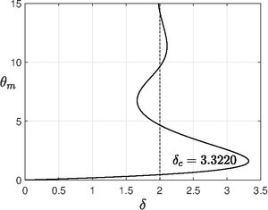
The above equation is nothing but Emden–Chandrasekhar equation, which appears in astrophysics describing isothermal gas sphere. Unlike planar and cylindrical case, the spherical vessel has infinitely many solutions for [math]\displaystyle{ \delta\lt \delta_c }[/math] oscillating about the point [math]\displaystyle{ \delta=2 }[/math], instead of just two solutions, which was shown by Israel Gelfand. The lowest branch will be chosen to explain explosive behavior.

From numerical solution, it is found that the critical Frank-Kamenetskii parameter is [math]\displaystyle{ \delta_c=3.3220 }[/math]. The system has no steady state( or explodes) for [math]\displaystyle{ \delta\gt \delta_c=3.3220 }[/math] and for [math]\displaystyle{ \delta\lt \delta_c=3.3220 }[/math], the system goes to a steady state with very slow reaction. The maximum temperature [math]\displaystyle{ \theta_m }[/math] occurs at [math]\displaystyle{ \eta=0 }[/math] and maximum critical temperature is [math]\displaystyle{ \theta_{m,c} = 1.6079 }[/math].

Non-symmetric geometries

For vessels which are not symmetric about the center (for example rectangular vessel), the problem involves solving a nonlinear partial differential equation instead of a nonlinear ordinary differential equation, which can be solved only through numerical methods in most cases. The equation is

[math]\displaystyle{ \nabla^2\theta + \delta e^\theta =0 }[/math]

with boundary condition [math]\displaystyle{ \theta=0 }[/math] on the bounding surfaces.

Applications

Since the model assumes homogeneous mixture, the theory is well applicable to study the explosive behavior of solid fuels (spontaneous ignition of bio fuels, organic materials, garbage, etc.,). This is also used to design explosives and fire crackers. The theory predicted critical values accurately for low conductivity fluids/solids with high conductivity thin walled containers.

See also

• Clarke's equation

External links

• The Frank-Kamenetskii problem in Wolfram solver http://demonstrations.wolfram.com/TheFrankKamenetskiiProblem/
• Tracking the Frank-Kamenetskii Problem in Wolfram solver http://demonstrations.wolfram.com/TrackingTheFrankKamenetskiiProblem/
• Planar solution in Chebfun solver http://www.chebfun.org/examples/ode-nonlin/BlowupFK.html

References

- ↑ Frank-Kamenetskii, David A. "Towards temperature distributions in a reaction vessel and the stationary theory of thermal explosion." Doklady Akademii Nauk SSSR. Vol. 18. 1938.
- ↑ Frank-Kamenetskii, D. A. "Calculation of thermal explosion limits." Acta. Phys.-Chim USSR 10 (1939): 365.
- ↑ Semenov, N. N. "The calculation of critical temperatures of thermal explosion." Z Phys Chem 48 (1928): 571.
- ↑ Semenov, N. N. "On the theory of combustion processes." Z. phys. Chem 48 (1928): 571–582.
- ↑ Frank-Kamenetskii, David Albertovich. Diffusion and heat exchange in chemical kinetics. Princeton University Press, 2015.
- ↑ Linan, Amable, and Forman Arthur Williams. "Fundamental aspects of combustion." (1993).
- ↑ Williams, Forman A. "Combustion theory." (1985).
- ↑ Buckmaster, John David, and Geoffrey Stuart Stephen Ludford. Theory of laminar flames. Cambridge University Press, 1982.
- ↑ Buckmaster, John D., ed. The mathematics of combustion. Society for Industrial and Applied Mathematics, 1985.
- ↑ Frank-Kamenetskii, D. A. (1946). The nonstationary theory of thermal explosion. Zhurnal fizichesko-khimii, 20, 139.
- ↑ Kassoy, D. R., & Linan, A. (1978). The influence of reactant consumption on the critical conditions for homogeneous thermal explosions. The Quarterly Journal of Mechanics and Applied Mathematics, 31(1), 99-112.
- ↑ Zeldovich, I. A., Barenblatt, G. I., Librovich, V. B., and Makhviladze, G. M. (1985). Mathematical theory of combustion and explosions.
- ↑ Lewis, Bernard, and Guenther Von Elbe. Combustion, flames and explosions of gases. Elsevier, 2012.
- ↑ Chambre, P. L. "On the Solution of the Poisson‐Boltzmann Equation with Application to the Theory of Thermal Explosions." The Journal of Chemical Physics 20.11 (1952): 1795–1797.
- ↑ Lemke, H. (1913). Über die Differentialgleichungen, welche den Gleichgewichtszustand eines gasförmigem Himmelskörpers bestimmen, dessen Teile gegeneinander nach dem Newtonschen Gesetz gravitieren. Journal für die reine und angewandte Mathematik, 142, 118-145.
- ↑ Subrahmanyan Chandrasekhar. An introduction to the study of stellar structure. Vol. 2. Courier Corporation, 1958.
- ↑ Jacobsen, Jon, and Klaus Schmitt. "The Liouville–Bratu–Gelfand problem for radial operators." Journal of Differential Equations 184.1 (2002): 283–298.
- ↑ Gelfand, I. M. (1963). Some problems in the theory of quasilinear equations. Amer. Math. Soc. Transl, 29(2), 295–381.
- ↑ Zukas, Jonas A., William Walters, and William P. Walters, eds. Explosive effects and applications. Springer Science & Business Media, 2002.