Randomised decision rule

In statistical decision theory, a randomised decision rule or mixed decision rule is a decision rule that associates probabilities with deterministic decision rules. In finite decision problems, randomised decision rules define a risk set which is the convex hull of the risk points of the nonrandomised decision rules. As nonrandomised alternatives always exist to randomised Bayes rules, randomisation is not needed in Bayesian statistics, although frequentist statistical theory sometimes requires the use of randomised rules to satisfy optimality conditions such as minimax, most notably when deriving confidence intervals and hypothesis tests about discrete probability distributions.

A statistical test making use of a randomized decision rule is called a randomized test.

Definition and interpretation

Let [math]\displaystyle{ \mathcal D =\{d_1, d_2 ..., d_h\} }[/math] be a set of non-randomised decision rules with associated probabilities [math]\displaystyle{ p_1, p_2, ..., p_h }[/math]. Then the randomised decision rule [math]\displaystyle{ d^* }[/math] is defined as [math]\displaystyle{ \sum_{i = 1}^h p_i d_i }[/math] and its associated risk function [math]\displaystyle{ R(\theta, d^*) }[/math] is [math]\displaystyle{ \sum_{i = 1}^h p_i R(\theta, d_i) }[/math]. This rule can be treated as a random experiment in which the decision rules [math]\displaystyle{ d_1, ... ,d_h \in \mathcal D }[/math] are selected with probabilities [math]\displaystyle{ p_1, ... p_h }[/math] respectively.

Alternatively, a randomised decision rule may assign probabilities directly on elements of the actions space [math]\displaystyle{ \mathcal A }[/math] for each member of the sample space. More formally, [math]\displaystyle{ d^*(x, A) }[/math] denotes the probability that an action [math]\displaystyle{ a \in \mathcal A }[/math] is chosen. Under this approach, its loss function is also defined directly as: [math]\displaystyle{ \int_{A \in \mathcal A}d^*(x, A) L(\theta, A) dA }[/math].

The introduction of randomised decision rules thus creates a larger decision space from which the statistician may choose his decision. As non-randomised decision rules are a special case of randomised decision rules where one decision or action has probability 1, the original decision space [math]\displaystyle{ \mathcal D }[/math] is a proper subset of the new decision space [math]\displaystyle{ \mathcal D^* }[/math].

Selection of randomised decision rules

The extreme points of the risk set, denoted by empty circles, correspond to nonrandomised decision rules, whereas the thick lines denote the admissible decision rules.

As with nonrandomised decision rules, randomised decision rules may satisfy favourable properties such as admissibility, minimaxity and Bayes. This shall be illustrated in the case of a finite decision problem, i.e. a problem where the parameter space is a finite set of, say, [math]\displaystyle{ k }[/math] elements. The risk set, henceforth denoted as [math]\displaystyle{ \mathcal S }[/math], is the set of all vectors in which each entry is the value of the risk function associated with a randomised decision rule under a certain parameter: it contains all vectors of the form [math]\displaystyle{ (R(\theta_1, d^*), ... R(\theta_k, d^*)), d^* \in \mathcal D^* }[/math]. Note that by the definition of the randomised decision rule, the risk set is the convex hull of the risks [math]\displaystyle{ (R(\theta_1, d), ... R(\theta_k, d)), d \in \mathcal D }[/math].

In the case where the parameter space has only two elements [math]\displaystyle{ \theta_1 }[/math] and [math]\displaystyle{ \theta_2 }[/math], this constitutes a subset of [math]\displaystyle{ \mathbb R^2 }[/math], so it may be drawn with respect to the coordinate axes [math]\displaystyle{ R_1 }[/math] and [math]\displaystyle{ R_2 }[/math] corresponding to the risks under [math]\displaystyle{ \theta_1 }[/math] and [math]\displaystyle{ \theta_2 }[/math] respectively. An example is shown on the right.

Admissibility

An admissible decision rule is one that is not dominated by any other decision rule, i.e. there is no decision rule that has equal risk as or lower risk than it for all parameters and strictly lower risk than it for some parameter. In a finite decision problem, the risk point of an admissible decision rule has either lower x-coordinates or y-coordinates than all other risk points or, more formally, it is the set of rules with risk points of the form [math]\displaystyle{ (a, b) }[/math] such that [math]\displaystyle{ \{(R_1, R_2): R_1 \leq a, R_2 \leq b \} \cap \mathcal S = (a, b) }[/math]. Thus the left side of the lower boundary of the risk set is the set of admissible decision rules.

Minimax

A minimax Bayes rule is one that minimises the supremum risk [math]\displaystyle{ \sup_{\theta \in \Theta} R(\theta, d^*) }[/math] among all decision rules in [math]\displaystyle{ \mathcal D^* }[/math]. Sometimes, a randomised decision rule may perform better than all other nonrandomised decision rules in this regard.

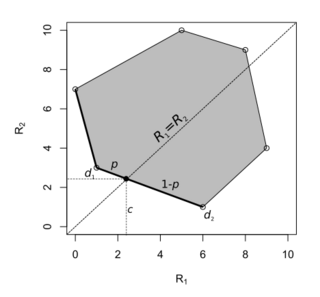
In a finite decision problem with two possible parameters, the minimax rule can be found by considering the family of squares [math]\displaystyle{ Q(c) = \{(R_1, R_2): 0 \leq R_1 \leq c, 0 \leq R_2 \leq c \} }[/math]. The value of [math]\displaystyle{ c }[/math] for the smallest of such squares that touches [math]\displaystyle{ \mathcal S }[/math] is the minimax risk and the corresponding point or points on the risk set is the minimax rule.

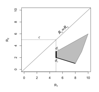
If the risk set intersects the line [math]\displaystyle{ R_1 = R_2 }[/math], then the admissible decision rule lying on the line is minimax. If [math]\displaystyle{ R_2 \gt R_1 }[/math] or [math]\displaystyle{ R_1 \gt R_2 }[/math] holds for every point in the risk set, then the minimax rule can either be an extreme point (i.e. a nonrandomised decision rule) or a line connecting two extreme points (nonrandomised decision rules).

• 

  The minimax rule is the randomised decision rule [math]\displaystyle{ (1-p)d_1 + pd_2 }[/math].

• 

  The minimax rule is [math]\displaystyle{ d_2 }[/math].

• 

  The minimax rules are all rules of the form [math]\displaystyle{ (1-p)d_1 + pd_2 }[/math], [math]\displaystyle{ 0 \leq p \leq 1 }[/math].

Bayes

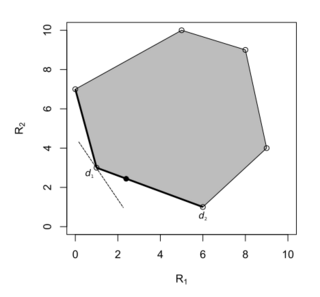
A randomised Bayes rule is one that has infimum Bayes risk [math]\displaystyle{ r(\pi, d^*) }[/math] among all decision rules. In the special case where the parameter space has two elements, the line [math]\displaystyle{ \pi_1 R_1 +(1 - \pi_1) R_2 = c }[/math], where [math]\displaystyle{ \pi_1 }[/math] and [math]\displaystyle{ \pi_2 }[/math] denote the prior probabilities of [math]\displaystyle{ \theta_1 }[/math] and [math]\displaystyle{ \theta_2 }[/math] respectively, is a family of points with Bayes risk [math]\displaystyle{ c }[/math]. The minimum Bayes risk for the decision problem is therefore the smallest [math]\displaystyle{ c }[/math] such that the line touches the risk set. This line may either touch only one extreme point of the risk set, i.e. correspond to a nonrandomised decision rule, or overlap with an entire side of the risk set, i.e. correspond to two nonrandomised decision rules and randomised decision rules combining the two. This is illustrated by the three situations below:

• 

  The Bayes rules are the set of decision rules of the form [math]\displaystyle{ (1-p)d_1 + pd_2 }[/math], [math]\displaystyle{ 0 \leq p \leq 1 }[/math].

• 

  The Bayes rule is [math]\displaystyle{ d_1 }[/math].

• 

  The Bayes rule is [math]\displaystyle{ d_2 }[/math].

As different priors result in different slopes, the set of all rules that are Bayes with respect to some prior are the same as the set of admissible rules.

Note that no situation is possible where a nonrandomised Bayes rule does not exist but a randomised Bayes rule does. The existence of a randomised Bayes rule implies the existence of a nonrandomised Bayes rule. This is also true in the general case, even with infinite parameter space, infinite Bayes risk, and regardless of whether the infimum Bayes risk can be attained. This supports the intuitive notion that the statistician need not utilise randomisation to arrive at statistical decisions.

In practice

As randomised Bayes rules always have nonrandomised alternatives, they are unnecessary in Bayesian statistics. However, in frequentist statistics, randomised rules are theoretically necessary under certain situations, and were thought to be useful in practice when they were first invented: Egon Pearson forecast that they 'will not meet with strong objection'. However, few statisticians actually implement them nowadays.

Randomised test

Not to be confused with Randomness test or Permutation test.

Randomized tests should not be confused with permutation tests.

In the usual formulation of the likelihood ratio test, the null hypothesis is rejected whenever the likelihood ratio [math]\displaystyle{ \Lambda }[/math] is smaller than some constant [math]\displaystyle{ K }[/math], and accepted otherwise. However, this is sometimes problematic when [math]\displaystyle{ \Lambda }[/math] is discrete under the null hypothesis, when [math]\displaystyle{ \Lambda = K }[/math] is possible.

A solution is to define a test function [math]\displaystyle{ \phi(x) }[/math], whose value is the probability at which the null hypothesis is accepted:

[math]\displaystyle{ \phi(x) = \left\{ \begin{array}{l} 1 & \text{ if } \Lambda \gt K \\ p(x) & \text{ if } \Lambda = K \\ 0 & \text{ if } \Lambda \lt K \end{array} \right. }[/math]

This can be interpreted as flipping a biased coin with a probability [math]\displaystyle{ p(x) }[/math] of returning heads whenever [math]\displaystyle{ \Lambda = k }[/math] and rejecting the null hypothesis if a heads turns up.

A generalised form of the Neyman–Pearson lemma states that this test has maximum power among all tests at the same significance level [math]\displaystyle{ \alpha }[/math], that such a test must exist for any significance level [math]\displaystyle{ \alpha }[/math], and that the test is unique under normal situations.

As an example, consider the case where the underlying distribution is Bernoulli with probability [math]\displaystyle{ p }[/math], and we would like to test the null hypothesis [math]\displaystyle{ p \leq \lambda }[/math] against the alternative hypothesis [math]\displaystyle{ p \gt \lambda }[/math]. It is natural to choose some [math]\displaystyle{ k }[/math] such that [math]\displaystyle{ P(\hat{p} \gt k|H_0) = \alpha }[/math], and reject the null whenever [math]\displaystyle{ \hat{p} \gt k }[/math], where [math]\displaystyle{ \hat{p} }[/math] is the test statistic. However, to take into account cases where [math]\displaystyle{ \hat p = k }[/math] , we define the test function:

[math]\displaystyle{ \phi(x) = \left\{ \begin{array}{l} 1 & \text{ if } \hat{p} \gt k\\ \gamma & \text{ if } \hat{p} = k \\ 0 & \text{ if } \hat{p} \lt k \end{array} \right. }[/math]

where [math]\displaystyle{ \gamma }[/math] is chosen such that [math]\displaystyle{ P(\hat{p} \gt k|H_0) + \gamma P(\hat{p} = k|H_0) = \alpha }[/math].

Randomised confidence intervals

An analogous problem arises in the construction of confidence intervals. For instance, the Clopper-Pearson interval is always conservative because of the discrete nature of the binomial distribution. An alternative is to find the upper and lower confidence limits [math]\displaystyle{ U }[/math] and [math]\displaystyle{ L }[/math] by solving the following equations:

[math]\displaystyle{ \left\{ \begin{array}{l} Pr (\hat{p} \lt k|p = U) + \gamma P(\hat{p} = k|p = U) &= \alpha/2\\ Pr (\hat{p} \gt k|p = L) + \gamma P(\hat{p} = k|p = L) &= \alpha/2 \end{array} \right. }[/math]

where [math]\displaystyle{ \gamma }[/math] is a uniform random variable on (0, 1).

See also

• Mixed strategy
• Linear programming

Bibliography

• Agresti, Alan; Gottard, Anna (2005). "Comment: Randomized Confidence Intervals and the Mid-P Approach". Statistical Science 5 (4): 367–371. doi:10.1214/088342305000000403. http://users.stat.ufl.edu/~aa/articles/agresti_gottard_2005.pdf. 
• Bickel, Peter J.; Doksum, Kjell A. (2001). Mathematical statistics : basic ideas and selected topics (2nd ed.). Upper Saddle River, NJ: Prentice-Hall. ISBN 978-0138503635. 
• DeGroot, Morris H. (2004). Optimal statistical decisions. Hoboken, N.J: Wiley-Interscience. ISBN 978-0471680291. 
• Parmigiani, Giovanni; Inoue, Lurdes Y T (2009). Decision theory : principles and approaches. Chichester, West Sussex: John Wiley and Sons. ISBN 9780470746684. 
• Robert, Christian P (2007). The Bayesian choice : from decision-theoretic foundations to computational implementation. New York: Springer. ISBN 9780387715988. 
• Young, G.A.; Smith, R.L. (2005). Essentials of Statistical Inference. Cambridge: Cambridge University Press. ISBN 9780521548663.