Rosenbrock function

Short description: Function used as a performance test problem for optimization algorithms

Plot of the Rosenbrock function of two variables. Here [math]\displaystyle{ a=1, b=100 }[/math], and the minimum value of zero is at [math]\displaystyle{ (1,1) }[/math].

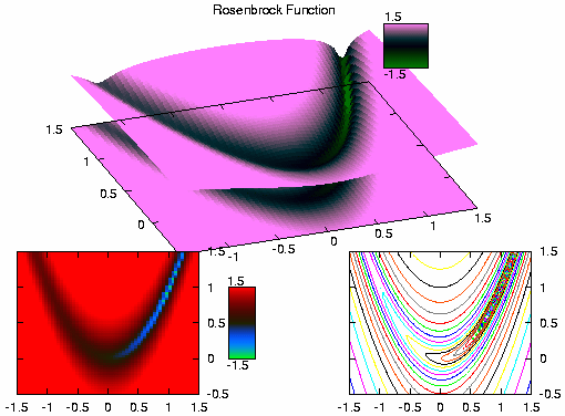
In mathematical optimization, the Rosenbrock function is a non-convex function, introduced by Howard H. Rosenbrock in 1960, which is used as a performance test problem for optimization algorithms. It is also known as Rosenbrock's valley or Rosenbrock's banana function.

The global minimum is inside a long, narrow, parabolic shaped flat valley. To find the valley is trivial. To converge to the global minimum, however, is difficult.

The function is defined by

[math]\displaystyle{ f(x, y) = (a-x)^2 + b(y-x^2)^2 }[/math]

It has a global minimum at [math]\displaystyle{ (x, y)=(a, a^2) }[/math], where [math]\displaystyle{ f(x, y)=0 }[/math]. Usually, these parameters are set such that [math]\displaystyle{ a = 1 }[/math] and [math]\displaystyle{ b = 100 }[/math]. Only in the trivial case where [math]\displaystyle{ a=0 }[/math] the function is symmetric and the minimum is at the origin.

Multidimensional generalizations

Two variants are commonly encountered.

Animation of Rosenbrock's function of three variables.

One is the sum of [math]\displaystyle{ N/2 }[/math] uncoupled 2D Rosenbrock problems, and is defined only for even [math]\displaystyle{ N }[/math]s:

[math]\displaystyle{ f(\mathbf{x}) = f(x_1, x_2, \dots, x_N) = \sum_{i=1}^{N/2} \left[100(x_{2i-1}^2 - x_{2i})^2 + (x_{2i-1} - 1)^2 \right]. }[/math]

This variant has predictably simple solutions.

A second, more involved variant is

[math]\displaystyle{ f(\mathbf{x}) = \sum_{i=1}^{N-1} [100 (x_{i+1} - x_i^2 )^2 + (1-x_i)^2] \quad \mbox{where} \quad \mathbf{x} = (x_1, \ldots, x_N) \in \mathbb{R}^N. }[/math]

has exactly one minimum for [math]\displaystyle{ N=3 }[/math] (at [math]\displaystyle{ (1, 1, 1) }[/math]) and exactly two minima for [math]\displaystyle{ 4 \le N \le 7 }[/math]—the global minimum at [math]\displaystyle{ (1, 1, ..., 1) }[/math] and a local minimum near [math]\displaystyle{ \hat{\mathbf{x}} = (-1, 1, \dots, 1) }[/math]. This result is obtained by setting the gradient of the function equal to zero, noticing that the resulting equation is a rational function of [math]\displaystyle{ x }[/math]. For small [math]\displaystyle{ N }[/math] the polynomials can be determined exactly and Sturm's theorem can be used to determine the number of real roots, while the roots can be bounded in the region of [math]\displaystyle{ |x_i| \lt 2.4 }[/math]. For larger [math]\displaystyle{ N }[/math] this method breaks down due to the size of the coefficients involved.

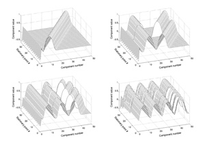
Stationary points

Many of the stationary points of the function exhibit a regular pattern when plotted. This structure can be exploited to locate them.

Rosenbrock roots exhibiting hump structures

Optimization examples

Nelder-Mead method applied to the Rosenbrock function

The Rosenbrock function can be efficiently optimized by adapting appropriate coordinate system without using any gradient information and without building local approximation models (in contrast to many derivate-free optimizers). The following figure illustrates an example of 2-dimensional Rosenbrock function optimization by adaptive coordinate descent from starting point [math]\displaystyle{ x_0=(-3,-4) }[/math]. The solution with the function value [math]\displaystyle{ 10^{-10} }[/math] can be found after 325 function evaluations.

Using the Nelder–Mead method from starting point [math]\displaystyle{ x_0=(-1,1) }[/math] with a regular initial simplex a minimum is found with function value [math]\displaystyle{ 1.36 \cdot 10^{-10} }[/math] after 185 function evaluations. The figure below visualizes the evolution of the algorithm.

See also

• Test functions for optimization

External links

• Rosenbrock function plot in 3D
• Weisstein, Eric W.. "Rosenbrock Function". http://mathworld.wolfram.com/RosenbrockFunction.html.

References

- ↑ Rosenbrock, H.H. (1960). "An automatic method for finding the greatest or least value of a function". The Computer Journal 3 (3): 175–184. doi:10.1093/comjnl/3.3.175. ISSN 0010-4620.
- ↑ Simionescu, P.A. (2014). Computer Aided Graphing and Simulation Tools for AutoCAD users (1st ed.). Boca Raton, FL: CRC Press. ISBN 978-1-4822-5290-3.
- ↑ Dixon, L. C. W.; Mills, D. J. (1994). "Effect of Rounding Errors on the Variable Metric Method". Journal of Optimization Theory and Applications 80: 175–179. doi:10.1007/BF02196600. http://portal.acm.org/citation.cfm?id=179711.
- ↑ "Generalized Rosenbrock's function". http://docs.scipy.org/doc/scipy-0.14.0/reference/tutorial/optimize.html#unconstrained-minimization-of-multivariate-scalar-functions-minimize.
- ↑ 5.0 5.1 Kok, Schalk; Sandrock, Carl (2009). "Locating and Characterizing the Stationary Points of the Extended Rosenbrock Function". Evolutionary Computation 17 (3): 437–53. doi:10.1162/evco.2009.17.3.437. PMID 19708775.
- ↑ Pagani, Filippo; Wiegand, Martin; Nadarajah, Saralees (2022). "An n-dimensional Rosenbrock distribution for Markov chain Monte Carlo testing" (in en). Scandinavian Journal of Statistics 49 (2): 657–680. doi:10.1111/sjos.12532. ISSN 1467-9469. https://onlinelibrary.wiley.com/doi/abs/10.1111/sjos.12532.