Software:Gekko (optimization software)

Short description: Python package

GEKKO

Developer(s)	Logan Beal and John Hedengren
Stable release	1.0.2 / December 2, 2021 (2021-12-02)
Operating system	Cross-Platform
Type	Technical computing
License	MIT
Website	gekko.readthedocs.io/en/latest/

The GEKKO Python package solves large-scale mixed-integer and differential algebraic equations with nonlinear programming solvers (IPOPT, APOPT, BPOPT, SNOPT, MINOS). Modes of operation include machine learning, data reconciliation, real-time optimization, dynamic simulation, and nonlinear model predictive control. In addition, the package solves Linear programming (LP), Quadratic programming (QP), Quadratically constrained quadratic program (QCQP), Nonlinear programming (NLP), Mixed integer programming (MIP), and Mixed integer linear programming (MILP). GEKKO is available in Python and installed with pip from PyPI of the Python Software Foundation.

pip install gekko

GEKKO works on all platforms and with Python 2.7 and 3+. By default, the problem is sent to a public server where the solution is computed and returned to Python. There are Windows, MacOS, Linux, and ARM (Raspberry Pi) processor options to solve without an Internet connection. GEKKO is an extension of the APMonitor Optimization Suite but has integrated the modeling and solution visualization directly within Python. A mathematical model is expressed in terms of variables and equations such as the Hock & Schittkowski Benchmark Problem #71 used to test the performance of nonlinear programming solvers. This particular optimization problem has an objective function [math]\displaystyle{ \min_{x\in\mathbb R}\; x_1 x_4 (x_1+x_2+x_3)+x_3 }[/math] and subject to the inequality constraint [math]\displaystyle{ x_1 x_2 x_3 x_4 \ge 25 }[/math] and equality constraint [math]\displaystyle{ {x_1}^2 + {x_2}^2 + {x_3}^2 + {x_4}^2=40 }[/math]. The four variables must be between a lower bound of 1 and an upper bound of 5. The initial guess values are [math]\displaystyle{ x_1 = 1, x_2=5, x_3=5, x_4=1 }[/math]. This optimization problem is solved with GEKKO as shown below.

from gekko import GEKKO

m = GEKKO()  # Initialize gekko
# Initialize variables
x1 = m.Var(value=1, lb=1, ub=5)
x2 = m.Var(value=5, lb=1, ub=5)
x3 = m.Var(value=5, lb=1, ub=5)
x4 = m.Var(value=1, lb=1, ub=5)
# Equations
m.Equation(x1 * x2 * x3 * x4 >= 25)
m.Equation(x1 ** 2 + x2 ** 2 + x3 ** 2 + x4 ** 2 == 40)
m.Obj(x1 * x4 * (x1 + x2 + x3) + x3)  # Objective
m.solve(disp=False)  # Solve
print("x1: " + str(x1.value))
print("x2: " + str(x2.value))
print("x3: " + str(x3.value))
print("x4: " + str(x4.value))
print("Objective: " + str(m.options.objfcnval))

Applications of GEKKO

Applications include cogeneration (power and heat), drilling automation, severe slugging control, solar thermal energy production, solid oxide fuel cells, flow assurance, Enhanced oil recovery, Essential oil extraction, and Unmanned Aerial Vehicles (UAVs). There are many other references to APMonitor and GEKKO as a sample of the types of applications that can be solved. GEKKO is developed from the National Science Foundation (NSF) research grant #1547110 and is detailed in a Special Issue collection on combined scheduling and control. Other notable mentions of GEKKO are the listing in the Decision Tree for Optimization Software, added support for APOPT and BPOPT solvers, projects reports of the online Dynamic Optimization course from international participants. GEKKO is a topic in online forums where users are solving optimization and optimal control problems. GEKKO is used for advanced control in the Temperature Control Lab (TCLab) for process control education at 20 universities.

Machine learning

Artificial Neural Network

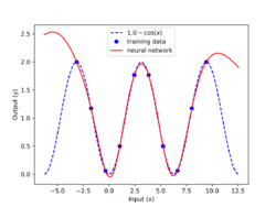
One application of machine learning is to perform regression from training data to build a correlation. In this example, deep learning generates a model from training data that is generated with the function [math]\displaystyle{ 1-\cos(x) }[/math]. An artificial neural network with three layers is used for this example. The first layer is linear, the second layer has a hyperbolic tangent activation function, and the third layer is linear. The program produces parameter weights that minimize the sum of squared errors between the measured data points and the neural network predictions at those points. GEKKO uses gradient-based optimizers to determine the optimal weight values instead of standard methods such as backpropagation. The gradients are determined by automatic differentiation, similar to other popular packages. The problem is solved as a constrained optimization problem and is converged when the solver satisfies Karush–Kuhn–Tucker conditions. Using a gradient-based optimizer allows additional constraints that may be imposed with domain knowledge of the data or system.

from gekko import brain
import numpy as np

b = brain.Brain()
b.input_layer(1)
b.layer(linear=3)
b.layer(tanh=3)
b.layer(linear=3)
b.output_layer(1)
x = np.linspace(-np.pi, 3 * np.pi, 20)
y = 1 - np.cos(x)
b.learn(x, y)

The neural network model is tested across the range of training data as well as for extrapolation to demonstrate poor predictions outside of the training data. Predictions outside the training data set are improved with hybrid machine learning that uses fundamental principles (if available) to impose a structure that is valid over a wider range of conditions. In the example above, the hyperbolic tangent activation function (hidden layer 2) could be replaced with a sine or cosine function to improve extrapolation. The final part of the script displays the neural network model, the original function, and the sampled data points used for fitting.

import matplotlib.pyplot as plt

xp = np.linspace(-2 * np.pi, 4 * np.pi, 100)
yp = b.think(xp)

plt.figure()
plt.plot(x, y, "bo")
plt.plot(xp, yp[0], "r-")
plt.show()

Optimal control

Optimal control problem benchmark (Luus) with an integral objective, inequality, and differential constraint.

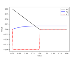
Optimal control is the use of mathematical optimization to obtain a policy that is constrained by differential [math]\displaystyle{ \left(\frac{d\,x_1}{d\,t}=u\right) }[/math], equality [math]\displaystyle{ \left(x_1(0) = 1\right) }[/math], or inequality [math]\displaystyle{ \left(-1 \le u(t) \le 1\right) }[/math] equations and minimizes an objective/reward function [math]\displaystyle{ \left(\min_u \frac{1}{2} \int_0^2 x_1^2(t) \, dt\right) }[/math]. The basic optimal control is solved with GEKKO by integrating the objective and transcribing the differential equation into algebraic form with orthogonal collocation on finite elements.

from gekko import GEKKO
import numpy as np
import matplotlib.pyplot as plt

m = GEKKO()  # initialize gekko
nt = 101
m.time = np.linspace(0, 2, nt)
# Variables
x1 = m.Var(value=1)
x2 = m.Var(value=0)
u = m.Var(value=0, lb=-1, ub=1)
p = np.zeros(nt)  # mark final time point
p[-1] = 1.0
final = m.Param(value=p)
# Equations
m.Equation(x1.dt() == u)
m.Equation(x2.dt() == 0.5 * x1 ** 2)
m.Obj(x2 * final)  # Objective function
m.options.IMODE = 6  # optimal control mode
m.solve()  # solve
plt.figure(1)  # plot results
plt.plot(m.time, x1.value, "k-", label=r"$x_1$")
plt.plot(m.time, x2.value, "b-", label=r"$x_2$")
plt.plot(m.time, u.value, "r--", label=r"$u$")
plt.legend(loc="best")
plt.xlabel("Time")
plt.ylabel("Value")
plt.show()

See also

• APMonitor and Python.

External links

• GEKKO Overview with Machine Learning and Optimization
• GEKKO Documentation
• GEKKO Source Code
• GEKKO on PyPI for Python pip install
• GEKKO is open-source product of National Science Foundation (NSF) research grant 1547110
• References to APMonitor and GEKKO in the literature
• 18 examples of GEKKO: machine learning, optimal control, data regression

References

- ↑ Beal, L. (2018). "GEKKO Optimization Suite". Processes 6 (8): 106. doi:10.3390/pr6080106.
- ↑ W. Hock and K. Schittkowski, Test Examples for Nonlinear Programming Codes, Lecture Notes in Economics and Mathematical Systems, Vol. 187, Springer 1981.
- ↑ Mojica, J. (2017). "Optimal combined long-term facility design and short-term operational strategy for CHP capacity investments". Energy 118: 97–115. doi:10.1016/j.energy.2016.12.009. https://scholarsarchive.byu.edu/facpub/1906.
- ↑ Eaton, A. (2017). "Real time model identification using multi-fidelity models in managed pressure drilling". Computers & Chemical Engineering 97: 76–84. doi:10.1016/j.compchemeng.2016.11.008.
- ↑ Eaton, A. (2015). "Post-installed fiber optic pressure sensors on subsea production risers for severe slugging control". OMAE 2015 Proceedings, St. John's, Canada. http://apm.byu.edu/prism/uploads/Projects/Eaton_OMAE15.pdf.
- ↑ Powell, K. (2014). "Dynamic Optimization of a Hybrid Solar Thermal and Fossil Fuel System". Solar Energy 108: 210–218. doi:10.1016/j.solener.2014.07.004. Bibcode: 2014SoEn..108..210P.
- ↑ Spivey, B. (2010). "Dynamic Modeling of Reliability Constraints in Solid Oxide Fuel Cells and Implications for Advanced Control". AIChE Annual Meeting Proceedings, Salt Lake City, Utah. http://apmonitor.com/wiki/uploads/Apps/sofc.pdf.
- ↑ Spivey, B. (2012). "Dynamic modeling, simulation, and MIMO predictive control of a tubular solid oxide fuel cell". Journal of Process Control 22 (8): 1502–1520. doi:10.1016/j.jprocont.2012.01.015.
- ↑ Hedengren, J. (2018). "New flow assurance system with high speed subsea fiber optic monitoring of pressure and temperature". ASME 37th International Conference on Ocean, Offshore and Arctic Engineering, OMAE2018/78079, Madrid, Spain. pp. V005T04A034. doi:10.1115/OMAE2018-78079. ISBN 978-0-7918-5124-1. https://scholarsarchive.byu.edu/cgi/viewcontent.cgi?article=3107&context=facpub.
- ↑ Udy, J. (2017). "Reduced order modeling for reservoir injection optimization and forecasting". FOCAPO / CPC 2017, Tucson, AZ. https://apm.byu.edu/prism/uploads/Members/udy2017_eor.pdf.
- ↑ Valderrama, F. (2018). "An optimal control approach to steam distillation of essential oils from aromatic plants". Computers & Chemical Engineering 117: 25–31. doi:10.1016/j.compchemeng.2018.05.009.
- ↑ Sun, L. (2013). "Optimal Trajectory Generation using Model Predictive Control for Aerially Towed Cable Systems". Journal of Guidance, Control, and Dynamics 37 (2): 525–539. doi:10.2514/1.60820. Bibcode: 2014JGCD...37..525S. http://apm.byu.edu/prism/uploads/Members/sun_2013.pdf.
- ↑ Beal, L. (2018). "Integrated scheduling and control in discrete-time with dynamic parameters and constraints". Computers & Chemical Engineering 115: 361–376. doi:10.1016/j.compchemeng.2018.04.010. https://scholarsarchive.byu.edu/facpub/2100.
- ↑ Beal, L. (2017). "Combined model predictive control and scheduling with dominant time constant compensation". Computers & Chemical Engineering 104: 271–282. doi:10.1016/j.compchemeng.2017.04.024. https://scholarsarchive.byu.edu/facpub/1905/.
- ↑ Beal, L. (2017). "Economic benefit from progressive integration of scheduling and control for continuous chemical processes". Processes 5 (4): 84. doi:10.3390/pr5040084. http://pdfs.semanticscholar.org/c5e3/0a7a866b83b659f118d161cc687d1b82cffc.pdf.
- ↑ Petersen, D. (2017). "Combined noncyclic scheduling and advanced control for continuous chemical processes". Processes 5 (4): 83. doi:10.3390/pr5040083. http://pdfs.semanticscholar.org/e2c7/f195a7a4f02b3e7b5df61abca2766a84b401.pdf.
- ↑ Hedengren, J. (2018). "Special issue: combined scheduling and control". Processes 6 (3): 24. doi:10.3390/pr6030024.
- ↑ Mittleman, Hans (1 May 2018). "Decision Tree for Optimization Software". Arizona State University. http://plato.asu.edu/sub/tools.html. "Object-oriented python library for mixed-integer and differential-algebraic equations"
- ↑ "Solver Solutions". Advanced Process Solutions, LLC. https://apopt.com. "GEKKO Python with APOPT or BPOPT Solvers"
- ↑ Everton, Colling. "Dynamic Optimization Projects". Petrobras, Statoil, Facebook. http://apmonitor.com/do/index.php/Main/ProjectLab. "Example Presentation: Everton Colling of Petrobras shares his experience with GEKKO for modeling and nonlinear control of distillation"
- ↑ "APMonitor Google Group: GEKKO". https://groups.google.com/forum/#!searchin/apmonitor/gekko.
- ↑ "Computational Science: Is there a high quality nonlinear programming solver for Python?". https://scicomp.stackexchange.com/questions/83/is-there-a-high-quality-nonlinear-programming-solver-for-python.
- ↑ Kantor, Jeff (2 May 2018). "TCLab Documentation". University of Notre Dame. https://media.readthedocs.org/pdf/tclab/stable/tclab.pdf. "pip install tclab"
- ↑ Kantor, Jeff (2 May 2018). "Chemical Process Control". University of Notre Dame. https://jckantor.github.io/CBE30338/. "Using the Temperature Control Lab (TCLab)"
- ↑ Hedengren, John (2 May 2018). "Advanced Temperature Control Lab". Brigham Young University. http://apmonitor.com/do/index.php/Main/AdvancedTemperatureControl. "Hands-on applications of advanced temperature control"
- ↑ Sandrock, Carl (2 May 2018). "Jupyter notebooks for Dynamics and Control". University of Pretoria, South Africa. https://github.com/alchemyst/Dynamics-and-Control. "CPN321 (Process Dynamics), and CPB421 (Process Control) at the Chemical Engineering department of the University of Pretoria"
- ↑ "CACHE News (Winter 2018): Incorporating Dynamic Simulation into Chemical Engineering Curricula". University of Texas at Austin. 2 May 2018. http://cache.org/files/winter-2018-dynamic-simulation.pdf. "Short Course at the ASEE 2017 Summer School hosted at SCSU by Hedengren (BYU), Grover (Georgia Tech), and Badgwell (ExxonMobil)"