Spatial heterogeneity

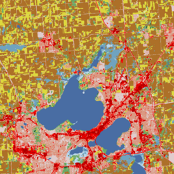
Spatial heterogeneity is a property generally ascribed to a landscape or to a population. It refers to the uneven distribution of various concentrations of each species within an area. A landscape with spatial heterogeneity has a mix of concentrations of multiple species of plants or animals (biological), or of terrain formations (geological), or environmental characteristics (e.g. rainfall, temperature, wind) filling its area. A population showing spatial heterogeneity is one where various concentrations of individuals of this species are unevenly distributed across an area; nearly synonymous with "patchily distributed."
Terminology
Spatial heterogeneity can be re-phrased as scaling hierarchy of far more small things than large ones. It has been formulated as a scaling law.[1]
Spatial heterogeneity or scaling hierarchy can be measured or quantified by ht-index: a head/tail breaks induced number. [2][3]
Examples
Environments with a wide variety of habitats such as different topographies, soil types, and climates are able to accommodate a greater amount of species. The leading scientific explanation for this is that when organisms can finely subdivide a landscape into unique suitable habitats, more species can coexist in a landscape without competition, a phenomenon termed "niche partitioning." Spatial heterogeneity is a concept parallel to ecosystem productivity, the species richness of animals is directly related to the species richness of plants in a certain habitat. Vegetation serves as food sources, habitats, and so on. Therefore, if vegetation is scarce, the animal populations will be as well. The more plant species there are in an ecosystem, the greater variety of microhabitats there are. Plant species richness directly reflects spatial heterogeneity in an ecosystem.
Types
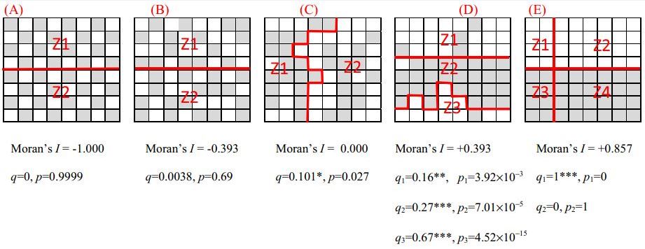
There exist two main types of spatial heterogeneity. The spatial local heterogeneity categorises the geographic phenomena whose its attributes' values are significantly similar within a directly local neighbourhood, but which significantly differ in the nearby surrounding-areas beyond this directly local neighbourhood (e.g. hot spots, cold spots). The spatial stratified heterogeneity categorises the geographic phenomena whose the within-strata variance of its attributes' values is significantly lower than its between-strata variance, such as collections of ecological zones or land-use classes within a given geographic area depict.[4]
Testing
Spatial local heterogeneity can be tested by LISA, Gi and SatScan, while spatial stratified heterogeneity of an attribute can be measured by geographical detector q-statistic:[4]
where a population is partitioned into h = 1, ..., L strata; N stands for the size of the population, σ2 stands for variance of the attribute. The value of q is within [0, 1], 0 indicates no spatial stratified heterogeneity, 1 indicates perfect spatial stratified heterogeneity. The value of q indicates the percent of the variance of an attribute explained by the stratification. The q follows a noncentral F probability density function.

Spatial heterogeneity for multivariate data and 3D data can also be statistically assessed using the "HTA index (HeTerogeneity Average index)". https://pypi.org/project/hta/.:[5]

Models
Spatial stratified heterogeneity
Optimal parameters-based geographical detector
Optimal Parameters-based Geographical Detector (OPGD) characterizes spatial heterogeneity with the optimized parameters of spatial data discretization for identifying geographical factors and interactive impacts of factors, and estimating risks.[6][7]
Interactive detector for spatial associations
Interactive Detector for Spatial Associations (IDSA) estimates power of interactive determinants (PID) on the basis of spatial stratified heterogeneity, spatial autocorrelation, and spatial fuzzy overlay of explanatory variables.[8]
Geographically optimal zones-based heterogeneity
Geographically Optimal Zones-based Heterogeneity (GOZH) explores individual and interactive determinants of geographical attributes (e.g., global soil moisture) across a large study area based on the identification of explainable geographically optimal zones.[9]
Robust geographical detector
Robust Geographical Detector (RGD) overcomes the limitation of the sensitivity in spatial data discretization and estimates robust power of determinants of explanatory variables.[10]
meta-STAR
The model-agnostic Spatial Transformation And modeRation (meta-STAR) is a framework for integrating the spatial heterogeneity into spatial statistical models (e.g. spatial ensemble methods, spatial neural networks), so to improve their accuracy. It involves the use of spatial networks/transformations and spatial moderators, plus handles the geo-spatial datasets representing geographic phenomena at multiple scales.[11]
Law of geography
In a 2004 publication titled "The Validity and Usefulness of Laws in Geographic Information Science and Geography," Michael Frank Goodchild proposed Spatial heterogeneity could be a candidate for a law of geography similar to Tobler's first law of geography.[12] The literature cites this paper and states this law as "geographic variables exhibit uncontrolled variance."[12][13][14] Often referred to as the second law of geography, or Michael Goodchild's second law of geography, it is one of many concepts competing for that term, including Tobler's second law of geography, and Arbia's law of geography.[13][14][15]
See also
References
- ↑ Jiang B. 2015. Geospatial analysis requires a different way of thinking: The problem of spatial heterogeneity. GeoJournal 80(1), 1–13.
- ↑ Jiang B. and Yin J. 2014. Ht-index for quantifying the fractal or scaling structure of geographic features, Annals of the Association of American Geographers, 104(3), 530–541.
- ↑ Jiang B. 2013. Head/tail breaks: A new classification scheme for data with a heavy-tailed distribution, The Professional Geographer, 65 (3), 482–494.
- ↑ 4.0 4.1 Wang JF, Zhang TL, Fu BJ. 2016. A measure of spatial stratified heterogeneity. Ecological Indicators 67: 250-256.
- ↑ 5.0 5.1 Alona Levy-Jurgenson and others, Assessing heterogeneity in spatial data using the HTA index with applications to spatial transcriptomics and imaging, Bioinformatics, Volume 37, Issue 21, November 2021, Pages 3796–3804, https://doi.org/10.1093/bioinformatics/btab569
- ↑ Song, Yongze; Wang, Jinfeng; Ge, Yong; Xu, Chengdong (2020). "An optimal parameters-based geographical detector model enhances geographic characteristics of explanatory variables for spatial heterogeneity analysis: cases with different types of spatial data" (in en). GIScience & Remote Sensing 57 (5): 593–610. doi:10.1080/15481603.2020.1760434. ISSN 1548-1603. https://www.tandfonline.com/doi/full/10.1080/15481603.2020.1760434.
- ↑ Song, Yongze (2021). "Optimal Parameters-based Geographical Detectors (OPGD) Model for Spatial Heterogeneity Analysis and Factor Exploration". https://cran.r-project.org/web/packages/GD/vignettes/GD.html.
- ↑ Song, Yongze; Wu, Peng (2021). "An interactive detector for spatial associations" (in en). International Journal of Geographical Information Science 35 (8): 1676–1701. doi:10.1080/13658816.2021.1882680. ISSN 1365-8816. https://www.tandfonline.com/doi/full/10.1080/13658816.2021.1882680.
- ↑ Luo, Peng; Song, Yongze; Huang, Xin; Ma, Hongliang; Liu, Jin; Yao, Yao; Meng, Liqiu (2022). "Identifying determinants of spatio-temporal disparities in soil moisture of the Northern Hemisphere using a geographically optimal zones-based heterogeneity model" (in en). ISPRS Journal of Photogrammetry and Remote Sensing 185: 111–128. doi:10.1016/j.isprsjprs.2022.01.009. Bibcode: 2022JPRS..185..111L. https://linkinghub.elsevier.com/retrieve/pii/S0924271622000132.
- ↑ Zhang, Zehua; Song, Yongze; Wu, Peng (2022). "Robust geographical detector" (in en). International Journal of Applied Earth Observation and Geoinformation 109: 102782. doi:10.1016/j.jag.2022.102782.
- ↑ "Harnessing heterogeneity in space with statistically guided meta-learning". Knowledge and Information Systems 65 (6): 2699–2729. 2023. doi:10.1007/s10115-023-01847-0. PMID 37035130.
- ↑ 12.0 12.1 Goodchild, Michael (2004). "The Validity and Usefulness of Laws in Geographic Information Science and Geography". Annals of the Association of American Geographers 94 (2): 300–303. doi:10.1111/j.1467-8306.2004.09402008.x.
- ↑ 13.0 13.1 Zou, Muquan; Wang, Lizhen; Wu, Ping; Tran, Vanha (23 July 2022). "Mining Type-β Co-Location Patterns on Closeness Centrality in Spatial Data Sets". ISPRS Int. J. Geo-Inf. 11 (8): 418. doi:10.3390/ijgi11080418.
- ↑ 14.0 14.1 Zhang, Yu; Sheng, Wu; Zhao, Zhiyuan; Yang, Xiping; Fang, Zhixiang (30 January 2023). "An urban crowd flow model integrating geographic characteristics". Scientific Reports 13. doi:10.1038/s41598-023-29000-5.
- ↑ Tobler, Waldo (2004). "On the First Law of Geography: A Reply". Annals of the Association of American Geographers 94 (2): 304–310. doi:10.1111/j.1467-8306.2004.09402009.x. http://www.tandfonline.com/doi/abs/10.1111/j.1467-8306.2004.09402009.x. Retrieved 10 March 2022.
 |
