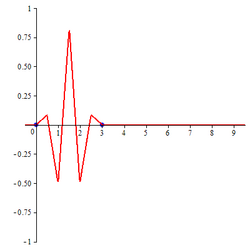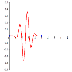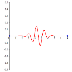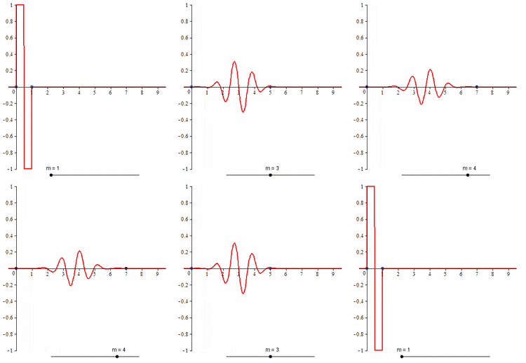
Spline wavelet

From HandWiki
Short description: Wavelet constructed using a spline function
Animation showing the compactly supported cardinal B-spline wavelets of orders 1, 2, 3, 4 and 5.

In the mathematical theory of wavelets, a spline wavelet is a wavelet constructed using a spline function.[1] There are different types of spline wavelets. The interpolatory spline wavelets introduced by C.K. Chui and J.Z. Wang are based on a certain spline interpolation formula.[2] Though these wavelets are orthogonal, they do not have compact supports. There is a certain class of wavelets, unique in some sense, constructed using B-splines and having compact supports. Even though these wavelets are not orthogonal they have some special properties that have made them quite popular.[3] The terminology spline wavelet is sometimes used to refer to the wavelets in this class of spline wavelets. These special wavelets are also called B-spline wavelets and cardinal B-spline wavelets.[4] The Battle-Lemarie wavelets are also wavelets constructed using spline functions.[5]

Cardinal B-splines

Let n be a fixed non-negative integer. Let Cn denote the set of all real-valued functions defined over the set of real numbers such that each function in the set as well its first n derivatives are continuous everywhere. A bi-infinite sequence . . . x−2, x−1, x0, x1, x2, . . . such that xr < xr+1 for all r and such that xr approaches ±∞ as r approaches ±∞ is said to define a set of knots. A spline of order n with a set of knots {xr} is a function S(x) in Cn such that, for each r, the restriction of S(x) to the interval [xr, xr+1) coincides with a polynomial with real coefficients of degree at most n in x.

If the separation xr+1 - xr, where r is any integer, between the successive knots in the set of knots is a constant, the spline is called a cardinal spline. The set of integers Z = {. . ., -2, -1, 0, 1, 2, . . .} is a standard choice for the set of knots of a cardinal spline. Unless otherwise specified, it is generally assumed that the set of knots is the set of integers.

A cardinal B-spline is a special type of cardinal spline. For any positive integer m the cardinal B-spline of order m, denoted by Nm(x), is defined recursively as follows.

[math]\displaystyle{ N_1(x)=\begin{cases}1 & 0\le x \lt 1 \\ 0 & \text{otherwise}\end{cases} }[/math]
[math]\displaystyle{ N_m(x)=\int_0^1 N_{m-1}(x-t)dt }[/math], for [math]\displaystyle{ m\gt 1 }[/math].

Concrete expressions for the cardinal B-splines of all orders up to 5 and their graphs are given later in this article.

Properties of the cardinal B-splines

Elementary properties

  1. The support of [math]\displaystyle{ N_m(x) }[/math] is the closed interval [math]\displaystyle{ [0,m] }[/math].
  2. The function [math]\displaystyle{ N_m(x) }[/math] is non-negative, that is, [math]\displaystyle{ N_m(x)\gt 0 }[/math] for [math]\displaystyle{ 0\lt x\lt m }[/math].
  3. [math]\displaystyle{ \sum_{k=-\infty}^\infty N_m(x-k)=1 }[/math] for all [math]\displaystyle{ x }[/math].
  4. The cardinal B-splines of orders m and m-1 are related by the identity: [math]\displaystyle{ N_m(x)=\frac{x}{m-1}N_{m-1}(x) + \frac{m-x}{m-1}N_{m-1}(x-1) }[/math].
  5. The function [math]\displaystyle{ N_m(x) }[/math] is symmetrical about [math]\displaystyle{ x=\frac{m}{2} }[/math], that is, [math]\displaystyle{ N_m\left(\frac{m}{2}-x\right)=N_m\left(\frac{m}{2}+x\right) }[/math].
  6. The derivative of [math]\displaystyle{ N_m(x) }[/math] is given by [math]\displaystyle{ N_m^\prime(x)=N_{m-1}(x)-N_{m-1}(x-1) }[/math].
  7. [math]\displaystyle{ \int_{-\infty}^\infty N_m(x)\, dx =1 }[/math]

Two-scale relation

The cardinal B-spline of order m satisfies the following two-scale relation:

[math]\displaystyle{ N_m(x)=\sum_{k=0}^m 2^{-m+1}{m \choose k}N_m(2x-k) }[/math].

Riesz property

The cardinal B-spline of order m satisfies the following property, known as the Riesz property: There exists two positive real numbers [math]\displaystyle{ A }[/math] and [math]\displaystyle{ B }[/math] such that for any square summable two-sided sequence [math]\displaystyle{ \{c_k\}_{k=-\infty}^\infty }[/math] and for any x,

[math]\displaystyle{ A \left\Vert \{c_k \} \right\Vert^2 \le \left \Vert \sum_{k=-\infty}^\infty c_k N_m(x-k) \right\Vert^2 \le B \left\Vert\{c_k\}\right\Vert^2 }[/math]

where [math]\displaystyle{ \Vert \cdot \Vert }[/math] is the norm in the ℓ2-space.

Cardinal B-splines of small orders

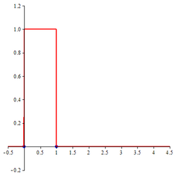
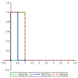
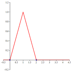
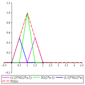
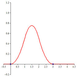
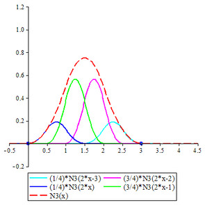
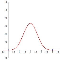
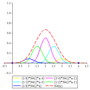
The cardinal B-splines are defined recursively starting from the B-spline of order 1, namely [math]\displaystyle{ N_1(x) }[/math], which takes the value 1 in the interval [0, 1) and 0 elsewhere. Computer algebra systems may have to be employed to obtain concrete expressions for higher order cardinal B-splines. The concrete expressions for cardinal B-splines of all orders up to 6 are given below. The graphs of cardinal B-splines of orders up to 4 are also exhibited. In the images, the graphs of the terms contributing to the corresponding two-scale relations are also shown. The two dots in each image indicate the extremities of the interval supporting the B-spline.

Constant B-spline

The B-spline of order 1, namely [math]\displaystyle{ N_1(x) }[/math], is the constant B-spline. It is defined by

[math]\displaystyle{ N_1(x)=\begin{cases}1 & 0\le x \lt 1 \\ 0 &\text{otherwise}\end{cases} }[/math]

The two-scale relation for this B-spline is

[math]\displaystyle{ N_1(x)=N_1(2x)+N_1(2x-1) }[/math]
Constant B-spline
[math]\displaystyle{ N_1(x) }[/math]
BSplineOfOrder1.png
TwoScaleRelationForBSplineOfOrder1.png

Linear B-spline

The B-spline of order 2, namely [math]\displaystyle{ N_2(x) }[/math], is the linear B-spline. It is given by

[math]\displaystyle{ N_2(x)=\begin{cases}x & 0\le x \lt 1 \\ -x+2 & 1\le x\lt 2 \\ 0 &\text{otherwise}\end{cases} }[/math]

The two-scale relation for this wavelet is

[math]\displaystyle{ N_2(x)=\frac{1}{2}N_2(2x)+N_2(2x-1)+\frac{1}{2}N_2(2x-2) }[/math]
Linear B-spline
[math]\displaystyle{ N_2(x) }[/math]
CardinalBSplineOfOrder2.png
TwoScaleRelationForCardinalBSplineOfOrder2.png

Quadratic B-spline

The B-spline of order 3, namely [math]\displaystyle{ N_3(x) }[/math], is the quadratic B-spline. It is given by

[math]\displaystyle{ N_3(x)= \begin{cases} \frac{1}{2}x^2 & 0\le x \lt 1 \\ -x^2 +3x-\frac{3}{2} & 1\le x\lt 2 \\ \frac{1}{2}x^2 -3x + \frac{9}{2} & 2\le x\lt 3 \\ 0 &\text{otherwise}\end{cases} }[/math]

The two-scale relation for this wavelet is

[math]\displaystyle{ N_3(x)=\frac{1}{4}N_3(2x)+\frac{3}{4}N_3(2x-1)+\frac{3}{4}N_3(2x-2)+\frac{1}{4}N_3(2x-3) }[/math]
Quadratic B-spline
[math]\displaystyle{ N_3(x) }[/math]
CardinalBSplineOfOrder3.png
TwoScaleRelationForCardinalBSplineOfOrder3.png

Cubic B-spline

The cubic B-spline is the cardinal B-spline of order 4, denoted by [math]\displaystyle{ N_4(x) }[/math]. It is given by the following expressions:

[math]\displaystyle{ N_4(x)= \begin{cases} \frac{1}{6}x^3 & 0\le x \lt 1 \\ -\frac{1}{2}x^3+2x^2-2x+\frac{2}{3} & 1\le x \lt 2 \\ \frac{1}{2}x^3-4x^2+10x-\frac{22}{3} & 2\le x\lt 3 \\ - \frac{1}{6}x^3 +2x^2 -8x +\frac{32}{3} & 3\le x \lt 4 \\ 0 & \text{otherwise} \end{cases} }[/math]

The two-scale relation for the cubic B-spline is

[math]\displaystyle{ N_4(x)=\frac{1}{8}N_4(2x)+\frac{1}{2}N_4(2x-1)+\frac{3}{4}N_4(2x-2)+\frac{1}{2}N_4(2x-3)+\frac{1}{8}N_4(2x-4) }[/math]
Cubic B-spline
[math]\displaystyle{ N_4(x) }[/math]
CardinalBSplineOfOrder4.png
TwoScaleRelationForCardinalBSplineOfOrder4 fixed.png

Bi-quadratic B-spline

The bi-quadratic B-spline is the cardinal B-spline of order 5 denoted by [math]\displaystyle{ N_5(x) }[/math]. It is given by

[math]\displaystyle{ N_5(x)= \begin{cases} \frac{1}{24}x^4 & 0 \le x \lt 1 \\ -\frac{1}{6}x^4+\frac{5}{6}x^3-\frac{5}{4}x^2 +\frac{5}{6}x-\frac{5}{24} & 1\le x \lt 2 \\ \frac{1}{4}x^4 -\frac{5}{2} x^3 +\frac{35}{4}x^2 -\frac{25}{2}x +\frac{155}{24} & 2\le x \lt 3 \\ -\frac{1}{6}x^4 +\frac{5}{2}x^3 -\frac{55}{4}x^2 +\frac{65}{2}x -\frac{655}{24} & 3 \le x \lt 4 \\ \frac{1}{24}x^4 - \frac{5}{6}x^3 + \frac{25}{4}x^2 - \frac{125}{6} x + \frac{625}{24} & 4 \le x \lt 5 \\ 0 & \text{otherwise} \end{cases} }[/math]

The two-scale relation is

[math]\displaystyle{ N_5(x)=\frac{1}{16}N_5(2x)+\frac{5}{16}N_5(2x-1)+\frac{10}{16}N_5(2x-2)+\frac{10}{16}N_5(2x-3)+\frac{5}{16}N_5(2x-4)+\frac{1}{16}N_5(2x-5) }[/math]

Quintic B-spline

The quintic B-spline is the cardinal B-spline of order 6 denoted by [math]\displaystyle{ N_6(x) }[/math]. It is given by

[math]\displaystyle{ N_6(x) = \begin{cases} \frac{1}{120}x^5 & 0\le x \lt 1 \\ -\frac{1}{24}x^5+\frac{1}{4}x^4 -\frac{1}{2}x^3 +\frac{1}{2}x^2 - \frac{1}{4}x +\frac{1}{20} & 1 \le x \lt 2 \\ \frac{1}{12}x^5 - x^4 +\frac{9}{2} x^3 -\frac{19}{2}x^2 +\frac{39}{4}x -\frac{79}{20} & 2 \le x \lt 3 \\ -\frac{1}{12}x^5 +\frac{3}{2}x^4 - \frac{21}{2}x^3 +\frac{71}{2}x^2 -\frac{231}{4}x+\frac{731}{20} & 3 \le x \lt 4 \\ \frac{1}{24}x^5 -x^4 +\frac{19}{2}x^3 - \frac{89}{2}x^2 +\frac{409}{4}x -\frac{1829}{20} & 4 \le x \lt 5 \\ -\frac{1}{120}x^5 +\frac{1}{4}x^4 -3x^3 +18x^2 -54 x +\frac{324}{5} & 5 \le x \lt 6 \\ 0 & \text{otherwise} \end{cases} }[/math]

Multi-resolution analysis generated by cardinal B-splines

The cardinal B-spline [math]\displaystyle{ N_m(x) }[/math] of order m generates a multi-resolution analysis. In fact, from the elementary properties of these functions enunciated above, it follows that the function [math]\displaystyle{ N_m(x) }[/math] is square integrable and is an element of the space [math]\displaystyle{ L^2(R) }[/math] of square integrable functions. To set up the multi-resolution analysis the following notations used.

  • For any integers [math]\displaystyle{ k,j }[/math], define the function [math]\displaystyle{ N_{m,kj}(x)=N_m(2^kx-j) }[/math].
  • For each integer [math]\displaystyle{ k }[/math], define the subspace [math]\displaystyle{ V_k }[/math] of [math]\displaystyle{ L^2(R) }[/math] as the closure of the linear span of the set [math]\displaystyle{ \{ N_{m,kj}(x): j=\cdots,-2,-1,0,1,2,\cdots\} }[/math].

That these define a multi-resolution analysis follows from the following:

  1. The spaces [math]\displaystyle{ V_k }[/math] satisfy the property: [math]\displaystyle{ \cdots \subset V_{-2}\subset V_{-1}\subset V_0 \subset V_1\subset V_2 \subset \cdots }[/math].
  2. The closure in [math]\displaystyle{ L^2(R) }[/math] of the union of all the subspaces [math]\displaystyle{ V_k }[/math] is the whole space [math]\displaystyle{ L^2(R) }[/math].
  3. The intersection of all the subspaces [math]\displaystyle{ V_k }[/math] is the singleton set containing only the zero function.
  4. For each integer [math]\displaystyle{ k }[/math] the set [math]\displaystyle{ \{N_{m,kj}(x): j= \cdots,-2,-1,0,1,2,\cdots\} }[/math] is an unconditional basis for [math]\displaystyle{ V_k }[/math]. (A sequence {xn} in a Banach space X is an unconditional basis for the space X if every permutation of the sequence {xn} is also a basis for the same space X.[6])

Wavelets from cardinal B-splines

Let m be a fixed positive integer and [math]\displaystyle{ N_m(x) }[/math] be the cardinal B-spline of order m. A function [math]\displaystyle{ \psi_m(x) }[/math] in [math]\displaystyle{ L^2(R) }[/math] is a basic wavelet relative to the cardinal B-spline function [math]\displaystyle{ N_m(x) }[/math] if the closure in [math]\displaystyle{ L^2(R) }[/math] of the linear span of the set [math]\displaystyle{ \{\psi_m(x-j):j=\cdots, -2,-1,0,1,2,\cdots\} }[/math] (this closure is denoted by [math]\displaystyle{ W_0 }[/math]) is the orthogonal complement of [math]\displaystyle{ V_0 }[/math] in [math]\displaystyle{ V_1 }[/math]. The subscript m in [math]\displaystyle{ \psi_m(x) }[/math] is used to indicate that [math]\displaystyle{ \psi_m(x) }[/math] is a basic wavelet relative the cardinal B-spline of order m. There is no unique basic wavelet [math]\displaystyle{ \psi_m(x) }[/math] relative to the cardinal B-spline [math]\displaystyle{ N_m(x) }[/math]. Some of these are discussed in the following sections.

Wavelets relative to cardinal B-splines using fundamental interpolatory splines

Fundamental interpolatory spline

Definitions

Let m be a fixed positive integer and let [math]\displaystyle{ N_m(x) }[/math] be the cardinal B-spline of order m. Given a sequence [math]\displaystyle{ \{f_j:j=\cdots, -2,-1,0,1,2,\cdots \} }[/math] of real numbers, the problem of finding a sequence [math]\displaystyle{ \{c_{m,k}: k=\cdots, -2,-1,0,1,2,\cdots \} }[/math] of real numbers such that

[math]\displaystyle{ \sum_{k=-\infty}^\infty c_{m,k} N_m\left(j+\frac{m}{2}-k\right) = f_j }[/math] for all [math]\displaystyle{ j }[/math],

is known as the cardinal spline interpolation problem. The special case of this problem where the sequence [math]\displaystyle{ \{f_j\} }[/math] is the sequence [math]\displaystyle{ \delta_{0j} }[/math], where [math]\displaystyle{ \delta_{ij} }[/math] is the Kronecker delta function [math]\displaystyle{ \delta_{ij} }[/math] defined by

[math]\displaystyle{ \delta_{ij}=\begin{cases}1,&\text{ if } i=j \\ 0, & \text{ if } i\ne j \end{cases} }[/math],

is the fundamental cardinal spline interpolation problem. The solution of the problem yields the fundamental cardinal interpolatory spline of order m. This spline is denoted by [math]\displaystyle{ L_m(x) }[/math] and is given by

[math]\displaystyle{ L_m(x) = \sum_{k=-\infty}^\infty c_{m,k} N_m\left(x+\frac{m}{2}-k\right) }[/math]

where the sequence [math]\displaystyle{ \{c_{m,k}\} }[/math] is now the solution of the following system of equations:

[math]\displaystyle{ \sum_{k=-\infty}^\infty c_{m,k} N_m\left(j+\frac{m}{2}-k\right) = \delta_{0j} }[/math]

Procedure to find the fundamental cardinal interpolatory spline

The fundamental cardinal interpolatory spline [math]\displaystyle{ L_m(x) }[/math] can be determined using Z-transforms. Using the following notations

[math]\displaystyle{ A(z)=\sum_{k=-\infty}^\infty \delta_{k0}z^k =1, }[/math]
[math]\displaystyle{ B_m(z)=\sum_{k=-\infty}^\infty N_m\left(k+\frac{m}{2}\right)z^k, }[/math]
[math]\displaystyle{ C_m(z)=\sum_{k=-\infty}^\infty c_{m,k} z^k, }[/math]

it can be seen from the equations defining the sequence [math]\displaystyle{ c_{m,k} }[/math] that

[math]\displaystyle{ B_m(z)C_m(z)=A(z) }[/math]

from which we get

[math]\displaystyle{ C_m(z)=\frac{1}{B_m(z)} }[/math].

This can be used to obtain concrete expressions for [math]\displaystyle{ c_{m,k} }[/math].

Example

As a concrete example, the case [math]\displaystyle{ L_4(x) }[/math] may be investigated. The definition of [math]\displaystyle{ B_m(z) }[/math] implies that

[math]\displaystyle{ B_4(x)=\sum_{k=-\infty}^\infty N_4(2+k)z^k }[/math]

The only nonzero values of [math]\displaystyle{ N_4(k+2) }[/math] are given by [math]\displaystyle{ k =-1,0,1 }[/math] and the corresponding values are

[math]\displaystyle{ N_4(1)= \frac{1}{6}, N_4(2) = \frac{4}{6}, N_4(3)=\frac{1}{6}. }[/math]

Thus [math]\displaystyle{ B_4(z) }[/math] reduces to

[math]\displaystyle{ B_4(z)=\frac{1}{6}z^{-1}+\frac{4}{6}z^0+\frac{1}{6}z^1=\frac{1+4z+z^2}{6z} }[/math]

This yields the following expression for [math]\displaystyle{ C_4(z) }[/math].

[math]\displaystyle{ C_4(z)=\frac{6z}{1+4z+z^2} }[/math]

Splitting this expression into partial fractions and expanding each term in powers of z in an annular region the values of [math]\displaystyle{ c_{4,k} }[/math] can be computed. These values are then substituted in the expression for [math]\displaystyle{ L_4(x) }[/math] to yield

[math]\displaystyle{ L_4(x)= \sum_{k=-\infty}^\infty (-1)^k \sqrt{3}(2-\sqrt{3})^{|k|}N_4(x+2-k) }[/math]

Wavelet using fundamental interpolatory spline

For a positive integer m, the function [math]\displaystyle{ \psi_m(x) }[/math] defined by

[math]\displaystyle{ \psi_{I,m}(x)=\frac{d^m}{dx^m}L_{2m}(2x-1) }[/math]

is a basic wavelet relative to the cardinal B-spline of order [math]\displaystyle{ N_m(x) }[/math]. The subscript I in [math]\displaystyle{ \psi_{I,m} }[/math] is used to indicate that it is based in the interpolatory spline formula. This basic wavelet is not compactly supported.

Example

The wavelet of order 2 using interpolatory spline is given by

[math]\displaystyle{ \psi_{I,2}(x)=\frac{d^2}{dx^2}L_4(2x-1) }[/math]

The expression for [math]\displaystyle{ L_4(x) }[/math] now yields the following formula:

[math]\displaystyle{ \psi_{I,2}(x)=\frac{d^2}{dx^2}\sum_{k=-\infty}^\infty (-1)^k \sqrt{3}(2-\sqrt{3})^{|k|}N_4(2x+1-k) }[/math]

Now, using the expression for the derivative of [math]\displaystyle{ N_m(x) }[/math] in terms of [math]\displaystyle{ N_{m-1}(x) }[/math] the function [math]\displaystyle{ \psi_2(x) }[/math] can be put in the following form:

[math]\displaystyle{ \psi_{I,2}(x)=\sum_{k=-\infty}^\infty (-1)^k 4 \sqrt{3}(2-\sqrt{3})^{|k|}\Big((N_2(2x+k-1)-2N_2(2x+k-2)+N_2(2x+k-3)\Big ) }[/math]

The following piecewise linear function is the approximation to [math]\displaystyle{ \psi_2(x) }[/math] obtained by taking the sum of the terms corresponding to [math]\displaystyle{ k=-3, \ldots, 3 }[/math] in the infinite series expression for [math]\displaystyle{ \psi_2(x) }[/math].

[math]\displaystyle{ \psi_{I,2}(x)\approx \begin{cases} 0.07142668x + 0.17856670 & -2.5\lt x \le -2 \\ -0.48084803 x -0.92598272 & -2 \lt x \le -1.5 \\ 2.0088293 x + 2.8085333 & -1.5 \lt x \le -1 \\ -7.5684795 x -6.7687755 & -1 \lt x \le - 0.5 \\ 28.245949 x + 11.138439 & -0.5 \lt x \le 0 \\ -57.415316 x + 11.138439& 0\lt x \le 0.5 \\ 57.415316 x -46.276878& 0.5 \lt x \le 1 \\ -28.245949x + 39.384388 & 1\lt x \le 1.5\\ 7.5684795 x-14.337255 & 1.5 \lt x \le 2\\ -2.0088293 x + 4.8173625 & 2 \lt x \le 2.5 \\ 0.48084803x -1.4068308& 2.5 \lt x \le 3\\ -0.07142668 x +0.24999338& 3 \lt x \le 3.5 \\ 0 & {otherwise} \end{cases} }[/math]

Two-scale relation

The two-scale relation for the wavelet function [math]\displaystyle{ \psi_m(x) }[/math] is given by

[math]\displaystyle{ \psi_{I,m}(x)=\sum_{-\infty}^\infty q_nN_m(2x-n) }[/math] where [math]\displaystyle{ q_n= \sum_{j=0}^m (-1)^j{m \choose j}c_{m+n-j-1}. }[/math]

Compactly supported B-spline wavelets

The spline wavelets generated using the interpolatory wavelets are not compactly supported. Compactly supported B-spline wavelets were discovered by Charles K. Chui and Jian-zhong Wang and published in 1991.[3][7] The compactly supported B-spline wavelet relative to the cardinal B-spline [math]\displaystyle{ N_m(x) }[/math] of order m discovered by Chui and Wong and denoted by [math]\displaystyle{ \psi_{C,m}(x) }[/math], has as its support the interval [math]\displaystyle{ [0, 2m-1] }[/math]. These wavelets are essentially unique in a certain sense explained below.

Definition

The compactly supported B-spline wavelet of order m is given by

[math]\displaystyle{ \psi_{C,m}(x)=\frac{1}{2^{m-1}}\sum_{j=0}^{2m-2} (-1)^j N_{2m}(j+1)\frac{d^m}{dx^m}N_{2m}(2x-j) }[/math]

This is an m-th order spline. As a special case, the compactly supported B-spline wavelet of order 1 is

[math]\displaystyle{ \psi_{C,1}(x)=N_2(1)\frac{d}{dx}N_2(2x) = \begin{cases}1 & 0\le x \lt \frac{1}{2} \\ -1 & \frac{1}{2} \le x \lt 1 \\ 0 & \text{otherwise}\end{cases} }[/math]

which is the well-known Haar wavelet.

Properties

  1. The support of [math]\displaystyle{ \psi_{C,m}(x) }[/math] is the closed interval [math]\displaystyle{ [0, 2m-1] }[/math].
  2. The wavelet [math]\displaystyle{ \psi_{C,m}(x) }[/math] is the unique wavelet with minimum support in the following sense: If [math]\displaystyle{ \eta(x) \in W_0 }[/math] generates [math]\displaystyle{ W_0 }[/math] and has support not exceeding [math]\displaystyle{ 2m-1 }[/math] in length then [math]\displaystyle{ \eta(x)=c_0\psi_{C,m}(x-n_0) }[/math] for some nonzero constant [math]\displaystyle{ c_0 }[/math] and for some integer [math]\displaystyle{ n_0 }[/math].[8]
  3. [math]\displaystyle{ \psi_{C,m}(x) }[/math] is symmetric for even m and antisymmetric for odd m.

Two-scale relation

[math]\displaystyle{ \psi_m(x) }[/math] satisfies the two-scale relation:

[math]\displaystyle{ \psi_{C,m}(x)=\sum_{n=0}^{3m-2}q_nN_m(2x-n) }[/math] where [math]\displaystyle{ q_n=\frac{(-1)^n}{2^{m-1}}\sum_{j=0}^m {m \choose j}N_{2m}(n-j+1) }[/math].

Decomposition relation

The decomposition relation for the compactly supported B-spline wavelet has the following form:

[math]\displaystyle{ N_m(2x-l) = \sum_{k=-\infty}^{\infty} \left[ a_{m, l-2k}N_m(x-k) + b_{m, l-2k}\psi_{C,m}(x-k)\right] }[/math]

where the coefficients [math]\displaystyle{ a_{m,j} }[/math] and [math]\displaystyle{ b_{m,j} }[/math] are given by

[math]\displaystyle{ a_{m,j}= - \frac{(-1)^j}{2}\sum_{l=-\infty}^\infty q_{-j+2m-2l+1}c_{2m,l}, }[/math]
[math]\displaystyle{ b_{m,j}= \frac{(-1)^j}{2}\sum_{l=-\infty}^\infty p_{-j+2m-2l+1}c_{2m,l}. }[/math]

Here the sequence [math]\displaystyle{ c_{2m,l} }[/math] is the sequence of coefficients in the fundamental interpolatoty cardinal spline wavelet of order m.

Compactly supported B-spline wavelets of small orders

Compactly supported B-spline wavelet of order 1

The two-scale relation for the compactly supported B-spline wavelet of order 1 is

[math]\displaystyle{ \psi_{C,1}(x)= N_1(2x)-N_1(2x-1) }[/math]

The closed form expression for compactly supported B-spline wavelet of order 1 is

[math]\displaystyle{ \psi_{C,1}(x)= \begin{cases} 1 & 0\le x \lt \frac{1}{2} \\ -1 & \frac{1}{2} \le x \lt 1\\ 0 & \text{otherwise} \end{cases} }[/math]

Compactly supported B-spline wavelet of order 2

The two-scale relation for the compactly supported B-spline wavelet of order 2 is

[math]\displaystyle{ \psi_{C,2}(x)= \frac{1}{12}\left(N_2(2x)-6 N_2(2x-1)+ 10 N_2(2x-2)-6 N_2(2x-3)+ N_2(2x-4)\right) }[/math]

The closed form expression for compactly supported B-spline wavelet of order 2 is

[math]\displaystyle{ \psi_{C,2}(x)= \begin{cases} \frac{1}{6}x & 0\le x \lt \frac{1}{2}\\ -\frac{7}{6}x + \frac{2}{3} & \frac{1}{2} \le x \lt 1\\ \frac{8}{3}x - \frac{19}{6} & 1 \le x \lt \frac{3}{2}\\ -\frac{8}{3} x + \frac{29}{6} & \frac{3}{2} \le x \lt 2 \\ \frac{7}{6} x- \frac{17}{6} & 2 \le x \lt \frac{5}{2}\\ -\frac{1}{6} x + \frac{1}{2} & \frac{5}{2} \le x \lt 3 \\ 0 & \text{otherwise} \end{cases} }[/math]

Compactly supported B-spline wavelet of order 3

The two-scale relation for the compactly supported B-spline wavelet of order 3 is

[math]\displaystyle{ \psi_{C,3}(x)= \frac{1}{480}\Big[ (N_3(2x)-29 N_3(2x-1)+ 147 N_3(2x-2)- 303 N_3(2x-3)+ }[/math]
[math]\displaystyle{ 303N_3(2x-4) - 147N_3(2x-5) + 29 N_3(2x-6) - N_3(2x-7)\Big] }[/math]

The closed form expression for compactly supported B-spline wavelet of order 3 is

[math]\displaystyle{ \psi_{C,3}(x)= \begin{cases} \frac{1}{240}x^2 & 0\le x \lt \frac{1}{2}\\ - \frac{31}{240}x^2+ \frac{2}{15}x- \frac{1}{30} & \frac{1}{2} \le x \lt 1\\ \frac{103}{120}x^2- \frac{221}{120}x + \frac{229}{240} & 1 \le x \lt \frac{3}{2}\\ -\frac{313}{120} x^2+ \frac{1027}{120}x- \frac{1643}{240} & \frac{3}{2} \le x \lt 2 \\ \frac{22}{5} x^2 - \frac{779}{40} x + \frac{339}{16} & 2 \le x \lt \frac{5}{2}\\ -\frac{22}{5} x^2 + \frac{981}{40} x- \frac{541}{16} & \frac{5}{2} \le x \lt 3 \\ \frac{313}{120}x^2-\frac{701}{40}x+ \frac{2341}{80 } & 3 \le x \lt \frac{7}{2} \\ -\frac{103}{120}x^2 +\frac{809}{120}x- \frac{3169}{240 } & \frac{7}{2} \le x \lt 4 \\ \frac{31}{240}x^2-\frac{139}{120}x+\frac{623}{240} & 4 \le x \lt \frac{9}{2} \\ -\frac{1}{240}x^2+\frac{1}{24}x-\frac{5}{48} & \frac{9}{2} \le x \lt 5 \\ 0 & \text{otherwise} \end{cases} }[/math]

Compactly supported B-spline wavelet of order 4

The two-scale relation for the compactly supported B-spline wavelet of order 4 is

[math]\displaystyle{ \psi_{C,4}(x)= \frac{1}{40320}\Big[ N_4(2x)- 124 N_4(2x-1)+ 1677 N_4(2x-2)- 7904 N_4(2x-3)+ 18482 N_4(2x-4) - }[/math]
[math]\displaystyle{ 24264 N_4(2x-5) + 18482N_4(2x-6) - 7904 N_4(2x-7) + 1677 N_4(2x-8) - 124N_4(2x-9) + N_4(2x-10)\Big] }[/math]

The closed form expression for compactly supported B-spline wavelet of order 4 is

[math]\displaystyle{ \psi_{C,4}(x)= \begin{cases} \frac{1}{30240}x^3 & 0\le x \lt \frac{1}{2}\\ -\frac{127}{30240}x^3+\frac{2}{315}x^2-\frac{1}{315}x+\frac{1}{1890 } & \frac{1}{2} \le x \lt 1\\ \frac{19}{280}x^3-\frac{47}{224}x^2+\frac{2147}{10080}x-\frac{103}{1440 } & 1 \le x \lt \frac{3}{2}\\ -\frac{1109}{2520}x^3+\frac{465}{224}x^2-\frac{32413}{10080}x+\frac{16559}{10080 } & \frac{3}{2} \le x \lt 2 \\ \frac{5261}{3360}x^3-\frac{33463}{3360}x^2+\frac{42043}{2016}x-\frac{145193}{10080} & 2 \le x \lt \frac{5}{2}\\ -\frac{35033}{10080}x^3+\frac{93577}{3360} x^2- \frac{148517}{2016}x+ \frac{216269}{3360} & \frac{5}{2} \le x \lt 3 \\ \frac{4832}{945}x^3- \frac{27691}{560}x^2+ \frac{113923}{720}x-\frac{28145}{168} & 3 \le x \lt \frac{7}{2} \\ -\frac{4832}{945}x^3+\frac{58393}{1008}x^2-\frac{52223}{240}x+\frac{2048227}{7560} & \frac{7}{2} \le x \lt 4 \\ \frac{35033}{10080}x^3-\frac{75827}{1680}x^2+\frac{981101}{5040}x- \frac{234149}{840} & 4 \le x \lt \frac{9}{2} \\ -\frac{5261}{3360}x^3+\frac{38509}{1680}x^2-\frac{112487}{1008}x+ \frac{30347}{168} & \frac{9}{2} \le x \lt 5 \\ \frac{1109}{2520}x^3-\frac{24077}{3360}x^2+\frac{78311}{2016}x- \frac{141311}{2016} & 5 \le x \lt \frac{11}{2} \\ -\frac{19}{280}x^3+\frac{1361}{1120}x^2-\frac{14617}{2016}x+\frac{4151}{288} & \frac{11}{2} \le x \lt 6 \\ \frac{127}{30240}x^3-\frac{55}{672}x^2+\frac{5359}{10080}x-\frac{11603}{10080} & 6 \le x \lt \frac{13}{2} \\ -\frac{1}{30240}x^3+\frac{1}{1440}x^2-\frac{7}{1440}x+ \frac{49}{4320} & \frac{13}{2} \le x \lt 7 \\ 0 & \text{otherwise} \end{cases} }[/math]

Compactly supported B-spline wavelet of order 5

The two-scale relation for the compactly supported B-spline wavelet of order 5 is

[math]\displaystyle{ \psi_{C,5}(x)= \frac{1}{5806080}\Big[N_5(2x)-507 N_5(2x-1)+17128 N_5(2x-2)-166304 N_5(2x-3)+ 748465N_5(2x-4) }[/math]
[math]\displaystyle{ -1900115N_5(2x-5)+2973560 N_5(2x-6)-2973560 N_5(2x-7)+1900115N_5(2x-8) }[/math]
[math]\displaystyle{ -748465 N_5(2x-9)+ 166304 N_5(2x-10)-17128N_5(2x-11)+507N_5(2x-12)-N_5(2x-13)\Big] }[/math]

The closed form expression for compactly supported B-spline wavelet of order 5 is

[math]\displaystyle{ \psi_{C,5}(x)= \begin{cases} \frac{1}{8709120}x^4 & 0\le x \lt \frac{1}{2} \\ - \frac{73}{1244160}x^4+\frac{1}{8505}x^3-\frac{1}{11340}x^2+\frac{1}{34020}x-\frac{1}{272160} & \frac{1}{2} \le x \lt 1 \\ \frac{9581}{4354560}x^4-\frac{19417}{2177280}x^3+\frac{1303}{96768}x^2-\frac{19609}{2177280}x+\frac{6547}{2903040} & 1\le x \lt \frac{3}{2} \\ -\frac{118931}{4354560}x^4+\frac{366119}{2177280}x^3-\frac{186253}{483840}x^2+\frac{121121}{311040}x-\frac{427181}{2903040} & \frac{3}{2} \le x \lt 2 \\ \frac{759239}{4354560}x^4-\frac{3146561}{2177280}x^3+\frac{6466601}{1451520}x^2-\frac{13202873}{2177280}x+\frac{26819897}{8709120} & 2\le x \lt \frac{5}{2} \\ -\frac{2980409}{4354560}x^4+\frac{5183893}{725760}x^3-\frac{13426333}{483840}x^2+\frac{426589}{8960}x-\frac{12635243}{414720} & \frac{5}{2}\le x \lt 3 \\ \frac{7873577}{4354560}x^4-\frac{16524079}{725760}x^3+\frac{7385369}{69120}x^2-\frac{17868671}{80640}x+\frac{497668543}{2903040} & 3\le x \lt \frac{7}{2} \\ - \frac{14714327}{4354560}x^4+\frac{108543091}{2177280}x^3-\frac{56901557}{207360}x^2+\frac{1454458651}{2177280}x-\frac{5286189059}{8709120} & \frac{7}{2}\le x \lt 4 \\ \frac{15619}{3402}x^4-\frac{33822017}{435456}x^3+\frac{15828929}{32256}x^2-\frac{597598433}{435456}x+\frac{277413649}{193536} & 4\le x \lt \frac{9}{2} \\ -\frac{15619}{3402}x^4+\frac{38150335}{435456}x^3-\frac{20157247}{32256}x^2+ \frac{859841695}{435456}x- \frac{64472345}{27648} &\frac{9}{2}\le x \lt 5 \\ \frac{14714327}{4354560}x^4-\frac{4466137}{62208}x^3+\frac{165651247}{290304}x^2-\frac{875490655}{435456}x+\frac{4614904015}{1741824} & 5\le x \lt \frac{11}{2} \\ -\frac{7873577}{4354560}x^4+\frac{30717383}{725760}x^3- \frac{179437319}{483840}x^2+ \frac{16606729}{11520}x- \frac{869722273}{414720} & \frac{11}{2}\le x \lt 6 \\ \frac{2980409}{4354560}x^4- \frac{12698561}{725760}x^3+ \frac{16211669}{96768}x^2-\frac{19138891}{26880}x+ \frac{3289787993}{2903040} & 6\le x \lt \frac{13}{2} \\ -\frac{759239}{4354560}x^4+\frac{10519741}{2177280}x^3- \frac{10403603}{207360}x^2+ \frac{71964499}{311040}x-\frac{3481646837}{8709120} & \frac{13}{2} \le x \lt 7 \\ \frac{118931}{4354560}x^4-\frac{1774639}{2177280}x^3+\frac{630259}{69120}x^2-\frac{14096161}{311040}x+\frac{245108501}{2903040} & 7\le x \lt \frac{15}{2} \\ -\frac{9581}{4354560}x^4+\frac{21863}{311040}x^3-\frac{407387}{483840}x^2+\frac{9758873}{2177280}x-\frac{25971499}{2903040} & \frac{15}{2} \le x \lt 8 \\ \frac{73}{1244160}x^4-\frac{4343}{2177280}x^3+ \frac{5273}{207360}x^2-\frac{313703}{2177280}x+ \frac{380873}{1244160} & 8\le x \lt \frac{17}{2} \\ -\frac{1}{8709120}x^4+ \frac{1}{241920}x^3- \frac{1}{17920}x^2+\frac{3}{8960}x-\frac{27}{35840} & \frac{17}{2} \le x \lt 9\\ 0 & \text{otherwise} \end{cases} }[/math]

Images of compactly supported B-spline wavelets
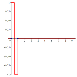
CardinalBSplineWaveletOfOrder1.png
CardinalBSplineWaveletOfOrder2.png
B-spline wavelet of order 1 B-spline wavelet of order 2
CardinalBSplineWaveletOfOrder3.png
center|250px
CardinalBSplineWaveletOfOrder5.png
B-spline wavelet of order 3 B-spline wavelet of order 4 B-spline wavelet of order 5

Battle-Lemarie wavelets

The Battle-Lemarie wavelets form a class of orthonormal wavelets constructed using the class of cardinal B-splines. The expressions for these wavelets are given in the frequency domain; that is, they are defined by specifying their Fourier transforms. The Fourier transform of a function of t, say, [math]\displaystyle{ F(t) }[/math], is denoted by [math]\displaystyle{ \hat{F}(\omega) }[/math].

Definition

Let m be a positive integer and let [math]\displaystyle{ N_m(x) }[/math] be the cardinal B-spline of order m. The Fourier transform of [math]\displaystyle{ N_m(x) }[/math] is [math]\displaystyle{ \hat{N}_m(\omega) }[/math]. The scaling function [math]\displaystyle{ \phi_m(t) }[/math] for the m-th order Battle-Lemarie wavelet is that function whose Fourier transform is

[math]\displaystyle{ \hat{\phi}_m(\omega) = \frac{\hat{N}_m(\omega)}{\left(\sum_{k=-\infty}^\infty \vert \hat{N}_m(\omega +2\pi k) \vert^2\right)^{1/2}}. }[/math]

The m-th order Battle-Lemarie wavelet is the function [math]\displaystyle{ \psi_{BL,m}(t) }[/math] whose Fourier transform is

[math]\displaystyle{ \hat{\psi}_{BL,m}(\omega) = - \frac{e^{-i\omega/2}\,\, \overline{\hat{\phi}_m(\omega + 2\pi)}\,\,\hat{\phi}_m\left(\frac{\omega}{2}\right)}{\overline{ \hat{\phi}_m\left(\frac{\omega}{2}+\pi\right)}} }[/math]

References

  1. Michael Unser (1997). "Ten good reasons for using spline wavelets". Proc. SPIE Vol. 3169, Wavelets Applications in Signal and Image Processing V. Wavelet Applications in Signal and Image Processing V 3169: 422–431. doi:10.1117/12.292801. Bibcode1997SPIE.3169..422U. http://bigwww.epfl.ch/publications/unser9702.pdf. Retrieved 21 December 2014. 
  2. Chui, Charles K, and Jian-zhong Wang (1991). "A cardinal spline approach to wavelets". Proceedings of the American Mathematical Society 113 (3): 785–793. doi:10.2307/2048616. http://www.ams.org/journals/proc/1991-113-03/S0002-9939-1991-1077784-X/S0002-9939-1991-1077784-X.pdf. Retrieved 22 January 2015. 
  3. 3.0 3.1 Charles K. Chui and Jian-Zhong Wang (April 1992). "On Compactly Supported Spline Wavelets and a Duality Principle". Transactions of the American Mathematical Society 330 (2): 903–915. doi:10.1090/s0002-9947-1992-1076613-3. http://www.shsu.edu/~mth_jxw/pdfflies/CWTRAN.pdf. Retrieved 21 December 2014. 
  4. Charles K Chui (1992). An Introduction to Wavelets. Academic Press. p. 177. 
  5. Ingrid Daubechies (1992). Ten Lectures on Wavelets. Philadelphia: Society for Industrial and Applied Mathematics. pp. 146–153. ISBN 9780898712742. https://archive.org/details/tenlecturesonwav0000daub. 
  6. Christopher Heil (2011). A Basis Theory Primer. Birkhauser. pp. 177–188. ISBN 9780817646868. https://archive.org/details/basistheoryprime00chei. 
  7. Charles K Chui (1992). An Introduction to Wavelets. Academic Press. p. 249. 
  8. Charles K Chui (1992). An Introduction to Wavelets. Academic Press. p. 184. 

Further reading