Studentized range distribution

Studentized range distribution

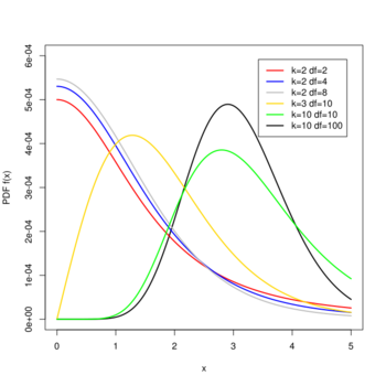
Probability density function
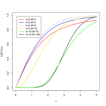
Cumulative distribution function
Parameters	k > 1, the number of groups [math]\displaystyle{ \nu }[/math] > 0, the degrees of freedom
Support	[math]\displaystyle{ q \in (0, +\infty) }[/math]
PDF	[math]\displaystyle{ \begin{matrix} f_\text{R}(q;k,\nu)=\frac{\,\sqrt{2\pi\,}\,k\,(k-1)\,\nu^{\nu/2}\,}{\Gamma(\nu/2)\,2^{\left(\nu/2-1\right)}}\int_0^\infty s^\nu\,\varphi(\sqrt{\nu\,}\,s)\,\times\\[0.5em] \left[\int_{-\infty}^\infty \varphi(z+q\,s)\,\varphi(z)\, \left[\Phi(z+q\,s)-\Phi(z)\right]^{k-2} \, \mathrm{d}z\right] \, \mathrm{d}s\end{matrix} }[/math]
CDF	[math]\displaystyle{ \begin{matrix} F_\text{R}(q;k,\nu) = \frac{\,\sqrt{2\pi\,}\,k\,\nu^{\nu/2}\,}{\,\Gamma(\nu/2)\,2^{\left(\nu/2 - 1\right)}} \int_0^\infty s^{\nu-1}\,\varphi(\sqrt{\nu\,}\,s)\,\times\\[0.5em] \qquad\left[\int_{-\infty}^\infty \varphi(z)\,\left[\Phi(z+q\,s)-\Phi(z)\right]^{k-1} \, \mathrm{d}z\right]\,\mathrm{d}s\end{matrix} }[/math]

In probability and statistics, studentized range distribution is the continuous probability distribution of the studentized range of an i.i.d. sample from a normally distributed population.

Suppose that we take a sample of size n from each of k populations with the same normal distribution N(μ, σ²) and suppose that [math]\displaystyle{ \bar{y}_{\min} }[/math] is the smallest of these sample means and [math]\displaystyle{ \bar{y}_{\max} }[/math] is the largest of these sample means, and suppose s² is the pooled sample variance from these samples. Then the following statistic has a Studentized range distribution.

[math]\displaystyle{ q = \frac{\overline{y}_{\max} - \overline{y}_{\min}}{s/\sqrt{n\,}} }[/math]

Definition

Probability density function

Differentiating the cumulative distribution function with respect to q gives the probability density function.

[math]\displaystyle{ f_\text{R}(q;k,\nu) = \frac{\sqrt{2\pi\,}\,k\,(k-1)\,\nu^{\nu/2}}{\Gamma(\nu /2)\,2^{\left(\nu/2-1\right)}}\int_0^\infty s^\nu \, \varphi(\sqrt{\nu\,} \,s)\,\left[\int_{-\infty}^\infty \varphi(z+q\,s)\,\varphi(z)\, \left[\Phi(z+q\,s)-\Phi(z)\right]^{k-2} \, \mathrm{d}z\right] \, \mathrm{d}s }[/math]

Note that in the outer part of the integral, the equation

[math]\displaystyle{ \varphi(\sqrt{\nu\,}\,s) \, \sqrt{2\pi\,} = e^{-\left(\nu\, s^2/2\right)} }[/math]

was used to replace an exponential factor.

Cumulative distribution function

The cumulative distribution function is given by

[math]\displaystyle{ F_\text{R}(q;k,\nu) = \frac{\sqrt{2\pi\,}\,k\,\nu^{\nu/2}}{\,\Gamma(\nu/2)\,2^{(\nu/2-1)}\,} \int_0^\infty s^{\nu-1} \varphi(\sqrt{\nu\,}\,s) \left[\int_{-\infty}^\infty \varphi(z) \left[\Phi(z+q\,s)-\Phi(z)\right]^{k-1} \, \mathrm{d}z \right] \, \mathrm{d}s }[/math]

Special cases

If k is 2 or 3, the studentized range probability distribution function can be directly evaluated, where [math]\displaystyle{ \varphi(z) }[/math] is the standard normal probability density function and [math]\displaystyle{ \Phi(z) }[/math] is the standard normal cumulative distribution function.

[math]\displaystyle{ f_R(q;k=2) = \sqrt{2\,}\,\varphi\left(\,q/\sqrt{2\,}\right) }[/math]

[math]\displaystyle{ f_R(q;k=3) = 6 \sqrt{2\,}\, \varphi\left(\,q/\sqrt{2\,}\right)\left[\Phi\left( q / \sqrt{6\,} \right)-\tfrac{1}{2} \right] }[/math]

When the degrees of freedom approaches infinity the studentized range cumulative distribution can be calculated for any k using the standard normal distribution.

[math]\displaystyle{ F_R(q;k) = k\, \int_{-\infty}^\infty \varphi(z)\,\Bigl[\Phi(z+q)-\Phi(z)\Bigr]^{k-1} \, \mathrm{d}z = k\, \int_{-\infty}^\infty \,\Bigl[\Phi(z+q)-\Phi(z)\Bigr]^{k-1} \, \mathrm{d}\Phi(z) }[/math]

Applications

Critical values of the studentized range distribution are used in Tukey's range test.

The studentized range is used to calculate significance levels for results obtained by data mining, where one selectively seeks extreme differences in sample data, rather than only sampling randomly.

The Studentized range distribution has applications to hypothesis testing and multiple comparisons procedures. For example, Tukey's range test and Duncan's new multiple range test (MRT), in which the sample x₁, ..., x_n is a sample of means and q is the basic test-statistic, can be used as post-hoc analysis to test between which two groups means there is a significant difference (pairwise comparisons) after rejecting the null hypothesis that all groups are from the same population (i.e. all means are equal) by the standard analysis of variance.

Related distributions

When only the equality of the two groups means is in question (i.e. whether μ₁ = μ₂), the studentized range distribution is similar to the Student's t distribution, differing only in that the first takes into account the number of means under consideration, and the critical value is adjusted accordingly. The more means under consideration, the larger the critical value is. This makes sense since the more means there are, the greater the probability that at least some differences between pairs of means will be significantly large due to chance alone.

Derivation

The studentized range distribution function arises from re-scaling the sample range R by the sample standard deviation s, since the studentized range is customarily tabulated in units of standard deviations, with the variable q = ​^R⁄_s . The derivation begins with a perfectly general form of the distribution function of the sample range, which applies to any sample data distribution.

In order to obtain the distribution in terms of the "studentized" range q, we will change variable from R to s and q. Assuming the sample data is normally distributed, the standard deviation s will be χ distributed. By further integrating over s we can remove s as a parameter and obtain the re-scaled distribution in terms of q alone.

General form

For any probability density function f_X, the range probability density f_R is:

[math]\displaystyle{ f_R(r;k) = k\,(k-1)\int_{-\infty}^\infty f_X\left(t+\tfrac{1}{2} r\right)f_X \left(t - \tfrac{1}{2} r\right) \left[\int_{t-\tfrac{1}{2}r}^{t+\tfrac{1}{2} r} f_X(x) \, \mathrm{d}x\right]^{k-2} \, \mathrm{d}\,t }[/math]

What this means is that we are adding up the probabilities that, given k draws from a distribution, two of them differ by r, and the remaining k − 2 draws all fall between the two extreme values. If we change variables to u where [math]\displaystyle{ u=t-\tfrac{1}{2} r }[/math] is the low-end of the range, and define F_X as the cumulative distribution function of f_X, then the equation can be simplified:

[math]\displaystyle{ f_R(r;k) = k\,(k-1)\int_{-\infty}^\infty f_X(u+r)\, f_X(u)\, \left[\, F_X(u+r)-F_X(u)\, \right]^{k-2} \, \mathrm{d}\,u }[/math]

We introduce a similar integral, and notice that differentiating under the integral-sign gives

[math]\displaystyle{ \begin{align} \frac{\partial}{\partial r} & \left[ k\,\int_{-\infty}^\infty f_X(u)\, \Bigl[\, F_X(u+r)-F_X(u)\, \Bigr]^{k-1} \, \mathrm{d}\,u \right] \\[5pt] = {} & k\,(k-1)\int_{-\infty}^\infty f_X(u+r)\, f_X(u)\, \Bigl[\, F_X(u+r)-F_X(u)\, \Bigr]^{k-2} \, \mathrm{d}\,u \end{align} }[/math]

which recovers the integral above, so that last relation confirms

[math]\displaystyle{ \begin{align} F_R(r;k) & = k \int_{-\infty}^\infty f_X(u) \Bigl[\, F_X(u+r)-F_X(u)\, \Bigr]^{k-1} \, \mathrm{d}\,u \\ & = k \int_{-\infty}^\infty \Bigl[\, F_X(u+r)-F_X(u)\, \Bigr]^{k-1} \, \mathrm{d}\,F_X(u) \end{align} }[/math]

because for any continuous cdf

[math]\displaystyle{ \frac{\partial F_R(r;k)}{\partial r} = f_R(r;k) }[/math]

Special form for normal data

The range distribution is most often used for confidence intervals around sample averages, which are asymptotically normally distributed by the central limit theorem.

In order to create the studentized range distribution for normal data, we first switch from the generic f_X and F_X to the distribution functions φ and Φ for the standard normal distribution, and change the variable r to s·q, where q is a fixed factor that re-scales r by scaling factor s:

[math]\displaystyle{ f_R(q;k) = s\,k\,(k-1)\int_{-\infty}^\infty \varphi(u+sq) \varphi(u)\, \left[\, \Phi(u+sq) - \Phi(u) \right]^{k-2} \, \mathrm{d}u }[/math]

Choose the scaling factor s to be the sample standard deviation, so that q becomes the number of standard deviations wide that the range is. For normal data s is chi distributed and the distribution function f_S of the chi distribution is given by:

[math]\displaystyle{ f_S(s;\nu)\,\mathrm{d}s = \begin{cases} \dfrac{\nu^{\nu/2}\,s^{\nu-1} e^{-\nu\,s^2/2}\,}{2^{\left(\nu/2 - 1\right)} \Gamma(\nu/2)} \, \mathrm{d}s & \text{for }\, 0 \lt s \lt \infty, \\[4pt] 0 & \text{otherwise}. \end{cases} }[/math]

Multiplying the distributions f_R and f_S and integrating to remove the dependence on the standard deviation s gives the studentized range distribution function for normal data:

[math]\displaystyle{ f_R(q;k,\nu) = \frac{\nu^{\nu/2}\,k\,(k-1)}{2^{\left( \nu/2 - 1\right)} \Gamma(\nu/2)} \int_0^\infty s^\nu e^{-\nu s^2/2} \int_{-\infty}^\infty \varphi(u+sq)\, \varphi(u)\, \left[\, \Phi(u+sq) - \Phi(u) \right]^{k-2} \, \mathrm{d}u \,\mathrm{d}s }[/math]

where

q is the width of the data range measured in standard deviations,

ν is the number of degrees of freedom for determining the sample standard deviation, and

k is the number of separate averages that form the points within the range.

The equation for the pdf shown in the sections above comes from using

[math]\displaystyle{ e^{-\nu\,s^2/2} = \sqrt{2\pi\,}\,\varphi(\sqrt{\nu\,}\,s) }[/math]

to replace the exponential expression in the outer integral.

Further reading

• Pearson, E.S.; Hartley, H.O. (1942). "The probability integral of the range in samples of N observations from a normal population". Biometrika 32 (3): 301–310. doi:10.1093/biomet/32.3-4.309. 
• Hartley, H.O. (1942). "The range in random samples". Biometrika 32 (3): 334–348. doi:10.2307/2332137. 
• Dunlap, W.P.; Powell, R.S.; Konnerth, T.K. (1977). "A FORTRAN IV function for calculating probabilities associated with the studentized range statistic". Behavior Research Methods & Instrumentation 9 (4): 373–375. doi:10.3758/BF03202264. 

External links

• Table of critical values for the Studentized range distribution

References

- ↑ Lund, R.E.; Lund, J.R. (1983). "Algorithm AS 190: Probabilities and upper quantiles for the studentized range". Journal of the Royal Statistical Society 32 (2): 204–210.
- ↑ 2.0 2.1 McKay, A.T. (1933). "A note on the distribution of range in samples of n". Biometrika 25 (3): 415–420. doi:10.2307/2332292.
- ↑ "StatsExamples | table of Q distribution critical values for alpha=0.05". http://www.statsexamples.com/table-Q-distribution-0.05.html.
- ↑ Pearson & Hartley (1970, Section 14.2)