Chi distribution

From HandWiki
Short description: Probability distribution
chi
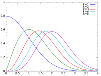
Probability density function
Plot of the Chi PMF
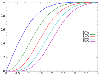
Cumulative distribution function
Plot of the Chi CMF
Parameters [math]\displaystyle{ k\gt 0\, }[/math] (degrees of freedom)
Support [math]\displaystyle{ x\in [0,\infty) }[/math]
PDF [math]\displaystyle{ \frac{1}{2^{(k/2)-1}\Gamma(k/2)}\;x^{k-1}e^{-x^2/2} }[/math]
CDF [math]\displaystyle{ P(k/2,x^2/2)\, }[/math]
Mean [math]\displaystyle{ \mu=\sqrt{2}\,\frac{\Gamma((k+1)/2)}{\Gamma(k/2)} }[/math]
Median [math]\displaystyle{ \approx \sqrt{k\bigg(1-\frac{2}{9k}\bigg)^3} }[/math]
Mode [math]\displaystyle{ \sqrt{k-1}\, }[/math] for [math]\displaystyle{ k\ge 1 }[/math]
Variance [math]\displaystyle{ \sigma^2=k-\mu^2\, }[/math]
Skewness [math]\displaystyle{ \gamma_1=\frac{\mu}{\sigma^3}\,(1-2\sigma^2) }[/math]
Kurtosis [math]\displaystyle{ \frac{2}{\sigma^2}(1-\mu\sigma\gamma_1-\sigma^2) }[/math]
Entropy [math]\displaystyle{ \ln(\Gamma(k/2))+\, }[/math]
[math]\displaystyle{ \frac{1}{2}(k\!-\!\ln(2)\!-\!(k\!-\!1)\psi_0(k/2)) }[/math]
MGF Complicated (see text)
CF Complicated (see text)

In probability theory and statistics, the chi distribution is a continuous probability distribution over the non-negative real line. It is the distribution of the positive square root of a sum of squared independent Gaussian random variables. Equivalently, it is the distribution of the Euclidean distance between a multivariate Gaussian random variable and the origin. It is thus related to the chi-squared distribution by describing the distribution of the positive square roots of a variable obeying a chi-squared distribution.

If [math]\displaystyle{ Z_1, \ldots, Z_k }[/math] are [math]\displaystyle{ k }[/math] independent, normally distributed random variables with mean 0 and standard deviation 1, then the statistic

[math]\displaystyle{ Y = \sqrt{\sum_{i=1}^k Z_i^2} }[/math]

is distributed according to the chi distribution. The chi distribution has one positive integer parameter [math]\displaystyle{ k }[/math], which specifies the degrees of freedom (i.e. the number of random variables [math]\displaystyle{ Z_i }[/math]).

The most familiar examples are the Rayleigh distribution (chi distribution with two degrees of freedom) and the Maxwell–Boltzmann distribution of the molecular speeds in an ideal gas (chi distribution with three degrees of freedom).

Definitions

Probability density function

The probability density function (pdf) of the chi-distribution is

[math]\displaystyle{ f(x;k) = \begin{cases} \dfrac{x^{k-1}e^{-x^2/2}}{2^{k/2-1}\Gamma\left(\frac{k}{2}\right)}, & x\geq 0; \\ 0, & \text{otherwise}. \end{cases} }[/math]

where [math]\displaystyle{ \Gamma(z) }[/math] is the gamma function.

Cumulative distribution function

The cumulative distribution function is given by:

[math]\displaystyle{ F(x;k)=P(k/2,x^2/2)\, }[/math]

where [math]\displaystyle{ P(k,x) }[/math] is the regularized gamma function.

Generating functions

The moment-generating function is given by:

[math]\displaystyle{ M(t)=M\left(\frac{k}{2},\frac{1}{2},\frac{t^2}{2}\right)+t\sqrt{2}\,\frac{\Gamma((k+1)/2)}{\Gamma(k/2)} M\left(\frac{k+1}{2},\frac{3}{2},\frac{t^2}{2}\right), }[/math]

where [math]\displaystyle{ M(a,b,z) }[/math] is Kummer's confluent hypergeometric function. The characteristic function is given by:

[math]\displaystyle{ \varphi(t;k)=M\left(\frac{k}{2},\frac{1}{2},\frac{-t^2}{2}\right) + it\sqrt{2}\,\frac{\Gamma((k+1)/2)}{\Gamma(k/2)} M\left(\frac{k+1}{2},\frac{3}{2},\frac{-t^2}{2}\right). }[/math]

Properties

Moments

The raw moments are then given by:

[math]\displaystyle{ \mu_j = \int_0^\infty f(x;k) x^j \mathrm{d} x = 2^{j/2}\ \frac{\ \Gamma\left( \tfrac{1}{2}(k+j) \right)\ }{\Gamma\left( \tfrac{1}{2}k \right)} }[/math]

where [math]\displaystyle{ \ \Gamma(z)\ }[/math] is the gamma function. Thus the first few raw moments are:

[math]\displaystyle{ \mu_1 = \sqrt{2\ }\ \frac{\ \Gamma\left( \tfrac{1}{2}(k + 1) \right)\ }{\Gamma\left( \tfrac{1}{2}k \right)} }[/math]
[math]\displaystyle{ \mu_2 = k\ , }[/math]
[math]\displaystyle{ \mu_3=2\sqrt{2\ }\ \frac{\ \Gamma\left( \tfrac{1}{2}(k + 3) \right)\ }{\Gamma\left( \tfrac{1}{2}k \right)} = (k+1)\ \mu_1\ , }[/math]
[math]\displaystyle{ \mu_4 = (k)(k+2)\ , }[/math]
[math]\displaystyle{ \mu_5 = 4\sqrt{2\ }\ \frac{\ \Gamma\left( \tfrac{1}{2}(k\!+\!5) \right)\ }{\Gamma\left( \tfrac{1}{2}k \right)} = (k+1)(k+3)\ \mu_1\ , }[/math]
[math]\displaystyle{ \mu_6 = (k)(k+2)(k+4)\ , }[/math]

where the rightmost expressions are derived using the recurrence relationship for the gamma function:

[math]\displaystyle{ \Gamma(x+1) = x\ \Gamma(x) ~. }[/math]

From these expressions we may derive the following relationships:

Mean: [math]\displaystyle{ \mu = \sqrt{2\ }\ \frac{\ \Gamma\left( \tfrac{1}{2}(k+1) \right)\ }{\Gamma\left( \tfrac{1}{2} k \right)}\ , }[/math] which is close to [math]\displaystyle{ \sqrt{k - \tfrac{1}{2}\ }\ }[/math] for large k.

Variance: [math]\displaystyle{ V = k - \mu^2\ , }[/math] which approaches [math]\displaystyle{ \ \tfrac{1}{2}\ }[/math] as k increases.

Skewness: [math]\displaystyle{ \gamma_1 = \frac{\mu}{\ \sigma^3\ } \left(1 - 2 \sigma^2 \right) ~. }[/math]

Kurtosis excess: [math]\displaystyle{ \gamma_2 = \frac{2}{\ \sigma^2\ } \left(1 - \mu\ \sigma\ \gamma_1 - \sigma^2 \right) ~. }[/math]

Entropy

The entropy is given by:

[math]\displaystyle{ S=\ln(\Gamma(k/2))+\frac{1}{2}(k\!-\!\ln(2)\!-\!(k\!-\!1)\psi^0(k/2)) }[/math]

where [math]\displaystyle{ \psi^0(z) }[/math] is the polygamma function.

Large n approximation

We find the large n=k+1 approximation of the mean and variance of chi distribution. This has application e.g. in finding the distribution of standard deviation of a sample of normally distributed population, where n is the sample size.

The mean is then:

[math]\displaystyle{ \mu = \sqrt{2}\,\,\frac{\Gamma(n/2)}{\Gamma((n-1)/2)} }[/math]

We use the Legendre duplication formula to write:

[math]\displaystyle{ 2^{n-2} \,\Gamma((n-1)/2)\cdot \Gamma(n/2) = \sqrt{\pi} \Gamma (n-1) }[/math],

so that:

[math]\displaystyle{ \mu = \sqrt{2/\pi}\,2^{n-2}\,\frac{(\Gamma(n/2))^2}{\Gamma(n-1)} }[/math]

Using Stirling's approximation for Gamma function, we get the following expression for the mean:

[math]\displaystyle{ \mu = \sqrt{2/\pi}\,2^{n-2}\,\frac{\left(\sqrt{2\pi}(n/2-1)^{n/2-1+1/2}e^{-(n/2-1)}\cdot[1+\frac{1}{12(n/2-1)}+O(\frac{1}{n^2})]\right)^2}{\sqrt{2\pi}(n-2)^{n-2+1/2}e^{-(n-2)}\cdot [1+\frac{1}{12(n-2)}+O(\frac{1}{n^2})]} }[/math]
[math]\displaystyle{ = (n-2)^{1/2}\,\cdot \left[1+\frac{1}{4n}+O(\frac{1}{n^2})\right] = \sqrt{n-1}\,(1-\frac{1}{n-1})^{1/2}\cdot \left[1+\frac{1}{4n}+O(\frac{1}{n^2})\right] }[/math]
[math]\displaystyle{ = \sqrt{n-1}\,\cdot \left[1-\frac{1}{2n}+O(\frac{1}{n^2})\right]\,\cdot \left[1+\frac{1}{4n}+O(\frac{1}{n^2})\right] }[/math]
[math]\displaystyle{ = \sqrt{n-1}\,\cdot \left[1-\frac{1}{4n}+O(\frac{1}{n^2})\right] }[/math]

And thus the variance is:

[math]\displaystyle{ V=(n-1)-\mu^2\, = (n-1)\cdot \frac{1}{2n}\,\cdot \left[1+O(\frac{1}{n})\right] }[/math]

Related distributions

Various chi and chi-squared distributions
Name Statistic
chi-squared distribution [math]\displaystyle{ \sum_{i=1}^k \left(\frac{X_i-\mu_i}{\sigma_i}\right)^2 }[/math]
noncentral chi-squared distribution [math]\displaystyle{ \sum_{i=1}^k \left(\frac{X_i}{\sigma_i}\right)^2 }[/math]
chi distribution [math]\displaystyle{ \sqrt{\sum_{i=1}^k \left(\frac{X_i-\mu_i}{\sigma_i}\right)^2} }[/math]
noncentral chi distribution [math]\displaystyle{ \sqrt{\sum_{i=1}^k \left(\frac{X_i}{\sigma_i}\right)^2} }[/math]

See also

References

  • Martha L. Abell, James P. Braselton, John Arthur Rafter, John A. Rafter, Statistics with Mathematica (1999), 237f.
  • Jan W. Gooch, Encyclopedic Dictionary of Polymers vol. 1 (2010), Appendix E, p. 972.

External links