Truncated distribution
|
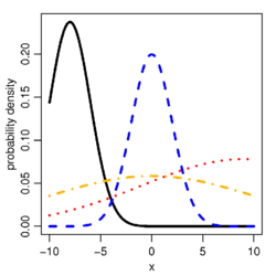
Probability density function  Probability density function for the truncated normal distribution for different sets of parameters. In all cases, a = −10 and b = 10. For the black: μ = −8, σ = 2; blue: μ = 0, σ = 2; red: μ = 9, σ = 10; orange: μ = 0, σ = 10. | |||
| Support | |||
|---|---|---|---|
| CDF | |||
| Mean | |||
| Median | |||
In statistics, a truncated distribution is a conditional distribution that results from restricting the domain of some other probability distribution. Truncated distributions arise in practical statistics in cases where the ability to record, or even to know about, occurrences is limited to values which lie above or below a given threshold or within a specified range. For example, if the dates of birth of children in a school are examined, these would typically be subject to truncation relative to those of all children in the area given that the school accepts only children in a given age range on a specific date. There would be no information about how many children in the locality had dates of birth before or after the school's cutoff dates if only a direct approach to the school were used to obtain information.
Where sampling is such as to retain knowledge of items that fall outside the required range, without recording the actual values, this is known as censoring, as opposed to the truncation here.[1]
Definition
The following discussion[2] is in terms of a random variable having a continuous distribution although the same ideas apply to discrete distributions. Similarly, the discussion assumes that truncation is to a semi-open interval y ∈ (a,b] but other possibilities can be handled straightforwardly.
Suppose we have a random variable, that is distributed according to some probability density function, , with cumulative distribution function both of which have infinite support. Suppose we wish to know the probability density of the random variable after restricting the support to be between two constants so that the support, . That is to say, suppose we wish to know how is distributed given .
where for all and everywhere else. That is, where is the indicator function. Note that the denominator in the truncated distribution is constant with respect to the .
Notice that in fact is a density:
- .
Truncated distributions need not have parts removed from the top and bottom. A truncated distribution where just the bottom of the distribution has been removed is as follows:
where for all and everywhere else, and is the cumulative distribution function.
A truncated distribution where the top of the distribution has been removed is as follows:
where for all and everywhere else, and is the cumulative distribution function.
Expectation of truncated random variable
Suppose we wish to find the expected value of a random variable distributed according to the density and a cumulative distribution of given that the random variable, , is greater than some known value . The expectation of a truncated random variable is thus:
where again is for all and everywhere else.
Letting and be the lower and upper limits respectively of support for the original density function (which we assume is continuous), properties of , where is some continuous function with a continuous derivative, include:
- and
Provided that the limits exist, that is: , and where represents either or .
Examples
The truncated normal distribution is an important example.[3] Literature has considered the left-truncated normal distribution,[4] the left-truncated Weibull distribution[5][6] and the left-truncated log-logistic distribution.[7]
The Tobit model employs truncated distributions. Other examples include truncated binomial at x=0 and truncated poisson at x=0.
Random truncation
Suppose we have the following set up: a truncation value, , is selected at random from a density, , but this value is not observed. Then a value, , is selected at random from the truncated distribution, . Suppose we observe and wish to update our belief about the density of given the observation.
First, by definition:
- , and
Notice that must be greater than , hence when we integrate over , we set a lower bound of . The functions and are the unconditional density and unconditional cumulative distribution function, respectively.
By Bayes' rule,
which expands to
Two uniform distributions (example)
Suppose we know that t is uniformly distributed from [0,T] and x|t is distributed uniformly on [0,t]. Let g(t) and f(x|t) be the densities that describe t and x respectively. Suppose we observe a value of x and wish to know the distribution of t given that value of x.
See also
References
- ↑ Dodge, Y. (2003) The Oxford Dictionary of Statistical Terms. OUP. ISBN 0-19-920613-9
- ↑ Kendall, Maurice G.; Stuart, Alan (1967). The Advanced Theory of Statistics Volume 2: Inference and Relationship (2nd ed.). London: Charles Griffin and Company Ltd., Section (32.17)
- ↑ Johnson, N.L., Kotz, S., Balakrishnan, N. (1994) Continuous Univariate Distributions, Volume 1, Wiley. ISBN 0-471-58495-9 (Section 10.1)
- ↑ del Castillo, Joan (March 1994). "The singly truncated normal distribution: A non-steep exponential family". Annals of the Institute of Statistical Mathematics 46 (1): 57–66. doi:10.1007/BF00773592. https://www.ism.ac.jp/editsec/aism/pdf/046_1_0057.pdf.
- ↑ Wingo, Dallas R. (December 1989). "The left-truncated Weibull distribution: theory and computation". Statistical Papers 30: 39–48. doi:10.1007/BF02924307. https://link.springer.com/article/10.1007/BF02924307.
- ↑ Kizilersu, Ayse; Kreer, Markus; Thomas, Anthony W. (June 2016). "Goodness-of-fit Testing for Left-truncated Two-parameter Weibull Distributions with Known Truncation point". Austrian Journal of Statistics 45 (3): 15–42. doi:10.17713/ajs.v45i3.106. https://www.ajs.or.at/index.php/ajs/article/view/doi%3A10.17713ajs.v45i3.106.
- ↑ Kreer, Markus; Kizilersu, Ayse; Guscott, Jake; Schmitz, Lukas Christopher; Thomas, Anthony W. (September 2024). "Maximum likelihood estimation for left-truncated log-logistic distributions with a given truncation point". Stastical Papers 65: 5409–5445. doi:10.1007/s00362-024-01603-8. https://link.springer.com/article/10.1007/s00362-024-01603-8.
 |
