Universal Functions Originator

Short description: Universal Functions Originator

Universal Functions Originator, or just UFO, is a new multi-purpose machine learning (ML) computing system that explains everything as pure mathematical equations. These expressions could be simple or highly complicated linear/nonlinear equations. Although the purpose of this technique is similar to that of classical symbolic regression (SR) algorithms, UFO works differently and it has its own mechanism, search space, and building strategy. For example, in UFO, each equation term (of intercepts, weights, exponents, arithmetic operators, and analytic functions) has its own search space and cannot be mixed with others. Also, UFO can be executed by any optimization algorithm, while SR algorithms require some special tree-based optimization algorithms; like genetic programming (GP).

Universal Functions Originator

UFO is designed by merging concepts taken from control systems, fuzzy systems, classical optimization, mixed-integer meta-heuristic optimization, and linear/nonlinear regression analysis. It is a multi-purpose computing system that can be used as an alternative to LR, NLR, ANNs, SVMs, and others. In UFO, everything is rendered as mathematical equations. The model structures are not constant where each term of arithmetic operators, analytic functions, and coefficients is subject to dynamic change until finding the optimal mathematical model. Some of the features that can be provided by UFO are:

• It can convert simple functions to highly complex mathematical equations, which might be used for some future applications; similar to encoding and decoding concepts.
• If applicable, UFO could simplify highly complex equations to some compact equivalent equations.
• It can act as a universal dual linear/nonlinear regression unit.
• It can be used to visualize high-dimensional functions.

Mechanism of Single Output Stream Structure

Suppose there is a data-set that consists of [math]\displaystyle{ n }[/math] predictors [math]\displaystyle{ \{x_1,x_2,\cdots,x_n\} }[/math] and one response [math]\displaystyle{ y }[/math]. If [math]\displaystyle{ y }[/math] is approximated by [math]\displaystyle{ \hat{y} }[/math], then the approximated response can be mathematically expressed as follows:

[math]\displaystyle{ \hat{y} = f(x_1,x_2,\cdots,x_k,x_{k+1},\cdots,x_{n-1},x_n) \ \ \ ; \ \ \ k=1,2,\cdots,n }[/math]

It can also be expressed using the following vector notation:

[math]\displaystyle{ \hat{y} = f(X) \ \ \ ; \ \ \ X=[x_1,x_2,\cdots,x_n] }[/math]

The difference between [math]\displaystyle{ y }[/math] and [math]\displaystyle{ \hat{y} }[/math] is called error ([math]\displaystyle{ \varepsilon }[/math]), which can be mathematically expressed as follows:

[math]\displaystyle{ y(X) = \hat{y}(X) + \varepsilon }[/math]

Figure 1: Feedback control system.

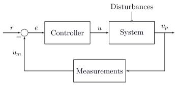
UFO can be understood as a feedback control system. Figure 1 shows the block diagram of feedback control loop. The objective of this control system is to let the controller adjust the process variable ([math]\displaystyle{ u_p }[/math]) to match with the set-point ([math]\displaystyle{ r }[/math]). The difference between [math]\displaystyle{ u_p }[/math] and [math]\displaystyle{ r }[/math] is the error of the control system ([math]\displaystyle{ e }[/math]), which can be calculated by subtracting the output of the measuring element ([math]\displaystyle{ u_m }[/math]) from the user-defined set-point ([math]\displaystyle{ r }[/math]). Mathematically speaking, the similarity here is:

[math]\displaystyle{ r \equiv y(X) \ \ , \ \ \ u_p \equiv \hat{y}(X) \ \ , \ \ \text{ and } \ \ e \equiv \varepsilon }[/math]

Now, let's take the following assumptions:

• The set-point is a set of values; i.e., [math]\displaystyle{ r }[/math] is a vector and not a scalar.
• The feedback stream is removed and [math]\displaystyle{ e }[/math] is minimized externally and instantaneously; i.e., without any delay between input and output.
• The interaction between blocks is not just a multiplication. Rather, it could be a multiplication, addition, subtraction, division, etc, or a mixture or set of them.
• There are [math]\displaystyle{ v }[/math] blocks inserted between [math]\displaystyle{ r }[/math] and [math]\displaystyle{ u_p }[/math].

Figure 2: Expressing UFO as a block diagram.

Thus, the structure shown in Figure 1 is modified to be something like the one shown in Figure 2. The thick arrows shown in Figure 2 mean that the system has a unidirectional flow of information, which is from the left side to the right side. Also, it tells us that the interaction between every two blocks is unknown. It could be a multiplication; similar to the feedback control loop shown in Figure 1. Alternatively, that interaction could also be made by using any standard or user-defined arithmetic operator; including addition, subtraction, and division.

If we suppose that the predicted response ([math]\displaystyle{ \hat{y} }[/math]) is decomposed into [math]\displaystyle{ v }[/math] blocks instead of just one block, then we will have the following:

[math]\displaystyle{ f \equiv \{f_1,f_2,\cdots,f_j,f_{j+1},\cdots,f_{v-1},f_v\} }[/math]

where each [math]\displaystyle{ j }[/math]th analytic function ([math]\displaystyle{ f_j }[/math]) could be taken from any of these categories:

• Basic Functions: [math]\displaystyle{ 1\times () }[/math], [math]\displaystyle{ \frac{1}{()} }[/math], [math]\displaystyle{ \sqrt{()} }[/math], [math]\displaystyle{ | \ | }[/math], [math]\displaystyle{ \lfloor \ \rfloor }[/math], [math]\displaystyle{ \lceil \ \rceil }[/math], [math]\displaystyle{ \lfloor \ \rceil }[/math], [math]\displaystyle{ \| \ \| }[/math], [math]\displaystyle{ ()! }[/math], [math]\displaystyle{ ()!! }[/math], [math]\displaystyle{ \cdots }[/math]
• Exponential/Logarithmic Functions: [math]\displaystyle{ \exp() }[/math], [math]\displaystyle{ \ln() }[/math], [math]\displaystyle{ \log_{10}() }[/math], [math]\displaystyle{ \log_2() }[/math], [math]\displaystyle{ \cdots }[/math]
• Trigonometric Functions: [math]\displaystyle{ \sin() }[/math], [math]\displaystyle{ \cos() }[/math], [math]\displaystyle{ \tan() }[/math], [math]\displaystyle{ \csc() }[/math], [math]\displaystyle{ \sec() }[/math], or [math]\displaystyle{ \cot() }[/math]
• Hyperbolic Functions: [math]\displaystyle{ \sinh() }[/math], [math]\displaystyle{ \cosh() }[/math], [math]\displaystyle{ \tanh() }[/math], [math]\displaystyle{ \mathrm{csch}() }[/math], [math]\displaystyle{ \mathrm{sech}() }[/math], or [math]\displaystyle{ \coth() }[/math]
• Inverse Trigonometric Functions: [math]\displaystyle{ \sin^{-1}() }[/math], [math]\displaystyle{ \cos^{-1}() }[/math], [math]\displaystyle{ \tan^{-1}() }[/math], [math]\displaystyle{ \csc^{-1}() }[/math], [math]\displaystyle{ \sec^{-1}() }[/math], or [math]\displaystyle{ \cot^{-1}() }[/math]
• Inverse Hyperbolic Functions: [math]\displaystyle{ \sinh^{-1}() }[/math], [math]\displaystyle{ \cosh^{-1}() }[/math], [math]\displaystyle{ \tanh^{-1}() }[/math], [math]\displaystyle{ \mathrm{csch}^{-1}() }[/math], [math]\displaystyle{ \mathrm{sech}^{-1}() }[/math], or [math]\displaystyle{ \coth^{-1}() }[/math]
• Unfamiliar Functions: [math]\displaystyle{ \mathrm{sinc}() }[/math], [math]\displaystyle{ \mathrm{versin}() }[/math], [math]\displaystyle{ \mathrm{vercos}() }[/math], [math]\displaystyle{ \mathrm{coversin}() }[/math], [math]\displaystyle{ \mathrm{covercos}() }[/math], [math]\displaystyle{ \mathrm{haversin}() }[/math], [math]\displaystyle{ \mathrm{havercos}() }[/math], [math]\displaystyle{ \mathrm{arcversin}() }[/math], [math]\displaystyle{ \mathrm{arcvercos}() }[/math], [math]\displaystyle{ \mathrm{arccoversin}() }[/math], [math]\displaystyle{ \mathrm{arccovercos}() }[/math], [math]\displaystyle{ \mathrm{archaversin}() }[/math], [math]\displaystyle{ \mathrm{archavercos}() }[/math], [math]\displaystyle{ \mathrm{hacoversin}() }[/math], [math]\displaystyle{ \mathrm{hacovercos}() }[/math], [math]\displaystyle{ \mathrm{exsec}() }[/math], [math]\displaystyle{ \mathrm{excsc}() }[/math], [math]\displaystyle{ \mathrm{si}() }[/math], [math]\displaystyle{ \mathrm{Si}() }[/math], [math]\displaystyle{ \mathrm{Ci}() }[/math], [math]\displaystyle{ \mathrm{Cin}() }[/math], [math]\displaystyle{ \mathrm{Shi}() }[/math], [math]\displaystyle{ \mathrm{Chi}() }[/math], [math]\displaystyle{ \cdots }[/math]
• User-Defined Functions

The interaction between the [math]\displaystyle{ n }[/math] independent variables or predictors in each [math]\displaystyle{ j }[/math]th analytic function can be modeled in many ways. The basic one is mathematically expressed as follows:

[math]\displaystyle{ f_j(X) = f_j\left(a_{0,j} \odot_{1,j} a_{1,j} \cdot x^{b_{1,j}}_1 \odot_{2,j} a_{2,j} \cdot x^{b_{2,j}}_2 \odot_{3,j} \ a_{3,j} \cdot x^{b_{3,j}}_3 \odot_{4,j} \cdots \odot_{n,j} a_{n,j} \cdot x^{b_{n,j}}_n\right) }[/math]

where:

• [math]\displaystyle{ \odot_{k,j} }[/math] is the [math]\displaystyle{ k }[/math]th arithmetic operator assigned to the [math]\displaystyle{ k }[/math]th predictor ([math]\displaystyle{ x_k }[/math]) of the [math]\displaystyle{ j }[/math]th block ([math]\displaystyle{ B_j }[/math]); it could be [math]\displaystyle{ + }[/math], [math]\displaystyle{ - }[/math], [math]\displaystyle{ \times }[/math], or [math]\displaystyle{ \div }[/math]
• [math]\displaystyle{ a_{0,j} }[/math] is the intercept of [math]\displaystyle{ B_j }[/math]; where [math]\displaystyle{ a_{0,j} \in [a^{\min}_{0,j},a^{\max}_{0,j}] }[/math]
• [math]\displaystyle{ a_{k,j} }[/math] is the [math]\displaystyle{ k }[/math]th internal weight assigned to [math]\displaystyle{ x_k }[/math] located in [math]\displaystyle{ B_j }[/math]; where [math]\displaystyle{ a_{k,j} \in [a^{\min}_{k,j},a^{\max}_{k,j}] }[/math]
• [math]\displaystyle{ b_{k,j} }[/math] is the [math]\displaystyle{ k }[/math]th internal exponent assigned to [math]\displaystyle{ x_k }[/math] located in [math]\displaystyle{ B_j }[/math]; where [math]\displaystyle{ b_{k,j} \in [b^{\min}_{k,j},b^{\max}_{k,j}] }[/math]

If each [math]\displaystyle{ f_j }[/math] has an external exponent ([math]\displaystyle{ c_j }[/math]) and the result is multiplied by an external weight ([math]\displaystyle{ w_j }[/math]), then the following more general function can be attained:

[math]\displaystyle{ \begin{matrix} g_j(X) &=& w_j \cdot \left[f_j(X)\right]^{c_j} = w_j \cdot \left[f_j(x_1,x_2,\cdots,x_n)\right]^{c_j} \ \ \ \ \ \ \ \ \ \ \ \ \ \ \ \ \ \ \ \ \ \ \ \ \ \ \ \ \ \ \ \ \ \ \ \ \ \ \ \ \ \ \ \ \ \ \ \ \ \ \ \ \ \ \ \ \ \ \ \ \ \ \ \ \ \ \ \ \ \ \ \ \\ &=& w_j \cdot \left[f_j\left(a_{0,j} \odot_{1,j} a_{1,j} \cdot x^{b_{1,j}}_1 \odot_{2,j} a_{2,j} \cdot x^{b_{2,j}}_2 \odot_{3,j} \ a_{3,j} \cdot x^{b_{3,j}}_3 \odot_{4,j} \cdots \odot_{n,j} a_{n,j} \cdot x^{b_{n,j}}_n\right)\right]^{c_j} \end{matrix} }[/math]

where:

• [math]\displaystyle{ c_j }[/math] is the external exponent assigned to [math]\displaystyle{ f_j }[/math] located in [math]\displaystyle{ B_j }[/math]; where [math]\displaystyle{ c_j \in [c^{\min}_{j},c^{\max}_{j}] }[/math]
• [math]\displaystyle{ w_j }[/math] is the external weight assigned to [math]\displaystyle{ B_j }[/math]; where [math]\displaystyle{ w_j \in [w^{\min}_j,w^{\max}_j] }[/math]

It has to be remembered that all the coefficients are not normalized. They could be normalized, but this action will reduce the explainability level of UFO.

The overall mathematical model expressed by UFO can then be expressed as follows:

[math]\displaystyle{ \hat{y}(X) = g_1(X) \circledcirc_1 g_2(X) \circledcirc_2 \cdots \circledcirc_{v-1} g_v(X) }[/math]

where [math]\displaystyle{ \{\circledcirc_1,\circledcirc_2,\cdots,\circledcirc_{v-1}\} }[/math] represent the interactions between the [math]\displaystyle{ v }[/math] blocks.

From the last two equations, both [math]\displaystyle{ \odot }[/math] and [math]\displaystyle{ \circledcirc }[/math] are identical. The first one is used between predictors and called the internal universal arithmetic operator, and the other is used between blocks and called the external universal arithmetic operator.

Figure 3: Illustrated UFO with only one O/P stream and universal arithmetic operators.

Although [math]\displaystyle{ \{a_{0,1},a_{0,2},\cdots,a_{0,v}\} }[/math] give UFO the ability to explain the constant term of the model, sometimes these internal intercepts serve as weights when [math]\displaystyle{ \{\odot_{1,1},\odot_{1,2},\cdots,\odot_{1,v}\} \in [\times,\div] }[/math]. Thus, an initial block [math]\displaystyle{ B_0 }[/math], which is also called the global block, is included in the UFO structure to have the following estimation:

[math]\displaystyle{ \hat{y}(X) = w_0 + g_1(X) \circledcirc_1 g_2(X) \circledcirc_2 \cdots \circledcirc_{v-1} g_v(X) }[/math]

where the scalar constant term [math]\displaystyle{ w_0 }[/math] can be called the model bias or the global constant term.

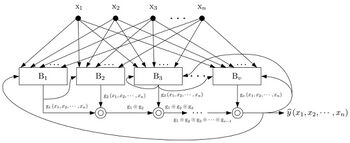
Merging all the information listed above leads us to the final single output stream UFO structure, which is shown in Figure 3.

Example

To clarify the last equations, let's take the following example:

How Does UFO Build Mathematical Models?

Suppose [math]\displaystyle{ v=3 }[/math], [math]\displaystyle{ n=4 }[/math], [math]\displaystyle{ f=[\mathrm{versin},\csc,\sqrt{ \ \ \ \ }] }[/math], [math]\displaystyle{ \odot_1 = [-,+,+,\div] }[/math], [math]\displaystyle{ \odot_2 = [\times,-,\times,+] }[/math], [math]\displaystyle{ \odot_3 = [\div,+,\times,-] }[/math], [math]\displaystyle{ \circledcirc_1 = + }[/math], and [math]\displaystyle{ \circledcirc_2 = \div }[/math]. The actual response ([math]\displaystyle{ y }[/math]) can be approximated as follows: [math]\displaystyle{ \hat{y}(X) = w_0 + g_1(X) + \frac{g_2(X)}{g_3(X)} }[/math] and each one of these block functions is expressed as follows: [math]\displaystyle{ g_1(X) = w_1 \cdot \left[\mathrm{versin}\left(a_{0,1} - a_{1,1} \cdot x_1^{b_{1,1}} + a_{2,1} \cdot x_2^{b_{2,1}} + \frac{a_{3,1} \cdot x_3^{b_{3,1}}}{a_{4,1} \cdot x_4^{b_{4,1}}}\right)\right]^{c_1} }[/math] [math]\displaystyle{ g_2(X) = w_2 \cdot \left[\csc\left(a_{0,2} \times a_{1,2} \cdot x_1^{b_{1,2}} - a_{2,2} \cdot x_2^{b_{2,2}} \times a_{3,2} \cdot x_3^{b_{3,2}} + a_{4,2} \cdot x_4^{b_{4,2}}\right)\right]^{c_2} }[/math] [math]\displaystyle{ g_3(X) = w_3 \cdot \left[\sqrt{\frac{a_{0,3}}{a_{1,3} \cdot x_1^{b_{1,3}}} + a_{2,3} \cdot x_2^{b_{2,3}} \times a_{3,3} \cdot x_3^{b_{3,3}} - a_{4,3} \cdot x_4^{b_{4,3}}}\right]^{c_3} }[/math] which ends up with the following final mathematical expression: [math]\displaystyle{ \hat{y}(X) = w_0 + w_1 \cdot \left[\mathrm{versin}\left(a_{0,1} - a_{1,1} \cdot x_1^{b_{1,1}} + a_{2,1} \cdot x_2^{b_{2,1}} + \frac{a_{3,1} \cdot x_3^{b_{3,1}}}{a_{4,1} \cdot x_4^{b_{4,1}}}\right)\right]^{c_1} + \frac{w_2 \cdot \left[\csc\left(a_{0,2} \times a_{1,2} \cdot x_1^{b_{1,2}} - a_{2,2} \cdot x_2^{b_{2,2}} \times a_{3,2} \cdot x_3^{b_{3,2}} + a_{4,2} \cdot x_4^{b_{4,2}}\right)\right]^{c_2}}{w_3 \cdot \left[\sqrt{\frac{a_{0,3}}{a_{1,3} \cdot x_1^{b_{1,3}}} + a_{2,3} \cdot x_2^{b_{2,3}} \times a_{3,3} \cdot x_3^{b_{3,3}} - a_{4,3} \cdot x_4^{b_{4,3}}}\right]^{c_3}} }[/math]

Main Stages

The mechanism of UFO is divided into four main stages:

• Pooling Stage: It is how the user can initialize UFO with his special requirement. He/she can define the set of analytic functions allowed to be in the final mathematical expression(s), the arithmetic operators between analytic functions and predictors, the side constraints or upper and lower limits of each continuous coefficient, and the chance to discretize these coefficients. Thus, the search space and the problem complexity depend on the settings defined in this stage.
• Building Stage: The preceding illustrative example is part of this stage. The user can use any mixed-integer optimization algorithm; even writing just a few lines of code to have a simple random search algorithm (RSA). However, it is preferred to use global meta-heuristic optimization algorithms because they are capable to search the entire search space for the global optimal or near-optimal solutions without using derivatives or matrices as faced with some classical local optimization algorithms.
• Tuning Stage: Once the functions are created in the building stage, the variables [math]\displaystyle{ \{f,\odot,\circledcirc\} }[/math] are kept unchanged, and then the tuning stage fine-tunes the remaining variables (i.e., [math]\displaystyle{ \{a_0,a,b,c,w\} }[/math]) by using a local optimization algorithm. Three possible options are available here:

1. Fine-tuning all the preceding numeric variables together by dealing with the problem as a nonlinear equation,
2. Fine-tuning all the preceding numeric variables separately by using a for-loop and then sequentially tuning them, or
3. Individually, by selecting one type of variables in each iteration (or for each candidate solution if a population-based optimization algorithm is used). That is, if only [math]\displaystyle{ w }[/math] is selected, then the whole stage can be quickly completed by dealing with the problem as a linear regression problem, which can be easily fine-tuned by using the ordinary least squares (OLS) algorithm. For [math]\displaystyle{ \{a,b\} }[/math], two sub-options are also available. For example, the user can fine-tune only the internal weight or exponent of only one or multiple predictors.

• Evaluation Stage: This optional stage is very useful to avoid the overfitting phenomenon, which can be done by dividing the original dataset into two sets (train and test sets) or three sets (train, validation, and test sets). Also, a part of this stage is responsible to visualize the results and export them in different shapes and formats.

Numerical Example

Consider the following problem from the Stack Overflow website. It asks to regress the following actual non-noisy response:

[math]\displaystyle{ y = \frac{1}{x} \ \ \ ; \ \ \ x \in [0.2,0.8] }[/math]

If UFO is used to evaluate this simple problem by using one analytic function (i.e., [math]\displaystyle{ v=1 }[/math]), then all the following mathematical equations are valid:

Regressing [math]\displaystyle{ \left(y = \frac{1}{x} \ \ \ ; \ \ \ x \in [0.2,0.8]\right) }[/math] via UFO
[math]\displaystyle{ \hat{y}(x) = 0.12432\times \left[-5.5877\times 10^{-10}+716.3481 x^{-3.1533}\right]^{0.31713} }[/math]	[math]\displaystyle{ \hat{y}(x) = 1\times\left[\frac{1}{\frac{153.286}{153.3842 x^1}}\right]^{-1} }[/math]
[math]\displaystyle{ \hat{y}(x) = 0.070685\times\left[\sqrt{2.0934\times 10^{-7}+811.4007 x^{-2.5283}}\right]^{0.79105} }[/math]	[math]\displaystyle{ \hat{y}(x) = 0.0064955\times\left[\exp\left(823.3554 - 818.3473 x^{0.0012166}\right)\right]^{1.0056} }[/math]
[math]\displaystyle{ \hat{y}(x) = 0.0045444\times\left[\log_{10}\left(1.0877 + 0.7281 x^{0.3679}\right)\right]^{-3.9957} }[/math]	[math]\displaystyle{ \hat{y}(x) = 0.42617\times\left[\ln\left(\frac{2990.6913}{8463.8354 x^{-1.1573}}\right)\right]^{-0.84314} }[/math]
[math]\displaystyle{ \hat{y}(x) = 0.47649\times\left[\sin\left(\frac{32.8572}{269.2354 x^{-2.838}}\right)\right]^{-0.35239} }[/math]	[math]\displaystyle{ \hat{y}(x) = 0.0091642\times\left[\cos\left(523.0655 - 0.30362 x^{0.26656}\right)\right]^{-3.9875} }[/math]
[math]\displaystyle{ \hat{y}(x) = 0.11809\times\left[\tan\left(\frac{43.0978}{908.674 x^{-1.4267}}\right)\right]^{-0.70084} }[/math]	[math]\displaystyle{ \hat{y}(x) = 0.43151\times\left[\csc\left(\frac{120.438}{991.1701 x^{-2.5085}}\right)\right]^{0.39868} }[/math]
[math]\displaystyle{ \hat{y}(x) = 0.0073526\times\left[\sec\left(-230.9069 - 0.085712 x^{0.49988}\right)\right]^{1.998} }[/math]	[math]\displaystyle{ \hat{y}(x) = 0.38785\times\left[\cot\left(\frac{60.8019}{903.7866 x^{-2.8493}}\right)\right]^{0.35094} }[/math]
[math]\displaystyle{ \hat{y}(x) = 0.43464\times\left[\sin^{-1}\left(\frac{88.6433}{574.0321 x^{-2.2405}}\right)\right]^{-0.44621} }[/math]	[math]\displaystyle{ \hat{y}(x) = \left(1.6314\times 10^{-19}\right) \left[\cos^{-1}\left(\frac{549.4935}{727.7463 x^{0.0047247}}\right)\right]^{-129} }[/math]
[math]\displaystyle{ \hat{y}(x) = 0.2713\times\left[\tan^{-1}\left(\frac{86.221}{949.0733 x^{-1.8397}}\right)\right]^{-0.54373} }[/math]	[math]\displaystyle{ \hat{y}(x) = 0.28349\times\left[\csc^{-1}\left(0.0004751 + 142.6188 x^{-3.9348}\right)\right]^{-0.25414} }[/math]
[math]\displaystyle{ \hat{y}(x) = 2835.957\times\left[\sec^{-1}\left(0.0025999 \left(741.9875 x^{0.0053775}\right)\right)\right]^{-311.4167} }[/math]	[math]\displaystyle{ \hat{y}(x) = 0.18829\times\left[\cot^{-1}\left(-0.00016689 + 794.7487 x^{-3.9994}\right)\right]^{-0.25004} }[/math]
[math]\displaystyle{ \hat{y}(x) = 0.7884\times\left[\sinh\left(\frac{106.6415}{816.441 x^{-8.5613}}\right)\right]^{-0.1168} }[/math]	[math]\displaystyle{ \hat{y}(x) = 0.48814\times\left[\cosh\left(-188.6685+ 186.7657 x^{0.0092334}\right)\right]^{0.58673} }[/math]
[math]\displaystyle{ \hat{y}(x) = 0.55786\times\left[\tanh\left(\frac{-130.247}{-935.4649 x^{-3.3793}}\right)\right]^{-0.29595} }[/math]	[math]\displaystyle{ \hat{y}(x) = 0.53903\times\left[\mathrm{csch}\left(\frac{145.0652}{881.8219 x^{-2.9193}}\right)\right]^{0.3425} }[/math]
[math]\displaystyle{ \hat{y}(x) = \left(2.4917\times 10^{-10}\right)\left[\mathrm{sech}\left(\frac{819.6646}{111.5549 x^{0.03936}}\right)\right]^{-3.3254} }[/math]	[math]\displaystyle{ \hat{y}(x) = 0.49314\times\left[\coth\left(\frac{44.0637}{636.8722 x^{-3.7783}}\right)\right]^{0.26468} }[/math]
[math]\displaystyle{ \hat{y}(x) = 0.35742\times\left[\sinh^{-1}\left(\frac{30.9341}{548.615 x^{-2.795}}\right)\right]^{-0.35779} }[/math]	[math]\displaystyle{ \hat{y}(x) = 0.92461\times\left[\cosh^{-1}\left(1.0889+0.47952 x^{-0.6276}\right)\right]^{3.9998} }[/math]
[math]\displaystyle{ \hat{y}(x) = 0.24526\times\left[\tanh^{-1}\left(\frac{86.2281}{996.3634 x^{-1.7402}}\right)\right]^{-0.57449} }[/math]	[math]\displaystyle{ \hat{y}(x) = 0.16828\times\left[\mathrm{csch}^{-1}\left(-8.9493\times 10^{-5} + 805.5713 x^{-3.7548}\right)\right]^{-0.26632} }[/math]
[math]\displaystyle{ \hat{y}(x) = \left(8.3719\times 10^{-8}\right)\left[\mathrm{sech}^{-1}\left(\frac{-312.9291}{-667.2605 x^{-0.025499}}\right)\right]^{49.4344} }[/math]	[math]\displaystyle{ \hat{y}(x) = 0.053339\times\left[\coth^{-1}\left(0.00030081 + 863.6727 x^{-2.3067}\right)\right]^{-0.43352} }[/math]

Mechanism of Recurrent One Output Stream Structure

Figure 4: Illustrated RUFO with only one O/P stream and universal arithmetic operators and without the global block.

The basic structure of UFO does not have any feedback stream. This has been seen during shifting from Figure 1 to Figure 2. Recurrent Universal Functions Originator, or just (RUFO), is a future design which considers some recurrent streams between blocks. Figure 4 shows one possible RUFO structure.

Mechanism of Multiple Output Streams Structure

Figure 5: Illustrated UFO with multiple O/P streams and universal arithmetic operators.

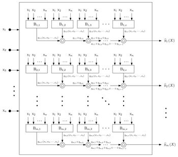
All the designs shown before have only one output stream. This means that UFO can accept only datasets with one response or target. Having multiple output UFO structures can be done by using any structure with/without recurrent streams. For example, if the basic structure shown in Figure 3 is used without the initial or global block [math]\displaystyle{ B_0 }[/math], then Figure 5 shows UFO with [math]\displaystyle{ m }[/math] responses.

UFO vs Other ML Tools

There are many differences between UFO and other machine learning computing systems. The following subsections list the major differences when UFO is compared with ANN and SR:

UFO vs ANNs

By comparing the mechanism of the basic UFO structure with ANNs, the following major differences can be highlighted:

• Neural networks have only weights and biases, while UFO has internal/external weights, internal/external exponents, and local/global intercepts. Moreover, except [math]\displaystyle{ w_0 }[/math], the other coefficients (i.e., [math]\displaystyle{ \{w,a_0,a,b,c\} }[/math]) could be just values or they can be even internal functions inside the main block functions; which could be considered for highly advanced UFO structures.
• The weights and biases in ANNs are normalized, while the coefficients of UFO are not. Add to that, [math]\displaystyle{ \{w,a_0,a,b,c\} }[/math] can be adjusted to be in a continuous or discrete mode.
• UFO has a built-in feature selection and function selection properties, which can be attained by setting some of the preceding coefficients to zero when they are on the discrete mode.
• For multiple output streams UFO structures, the interconnection between blocks of different rows is just an optional feature. On the opposite side, the interconnection between neurons is highly recommended.
• Once the number of blocks and data size are defined, the problem dimension remains unchanged in UFO. On the opposite side, the size of neural networks expanded with any increase in the number of neurons; even with fixing the number of hidden layers and the data size.
• It is well known that ANNs are black-boxes where the knowledge is distributed among neurons. In UFO, the explainability and interpretability criteria are highly satisfied by rendering everything as readable mathematical equations.
• ANNs are trained via one optimization algorithm, even with hybrid optimization algorithms. UFO uses two separate optimization algorithms, one as a mixed-integer in the building stage and the other as a mixed-integer or continuous in the tuning stage. Of course, some recent studies optimize the hyperparameters of ANNs via one additional external optimization algorithm. However, the other independent optimization algorithm is optional, while UFO is built through two mandatory independent optimization algorithms. Also, the hyperparameters of UFO can be optimized through one external optimization algorithm. This means that if ANNs have two optimization algorithms, then UFO will have three optimization algorithms.

UFO vs SRs

Although UFO and classical SR share the same aim, they are totally different. For example, let's refer to the study reported by Uy et al., the following differences can be highlighted:

• SRs depend on some special tree-based optimization algorithms, like GP, while UFO has a unique structure that lets it to work with any classical or meta-heuristic optimization algorithm; including the most primitive ones, like random search algorithm (RSA) that can be coded by just a few lines of code.
• The mathematical equations built by SRs have uncontrolled random expressions, while the expressions of UFO can be controlled by each [math]\displaystyle{ g_j(X) }[/math]. These [math]\displaystyle{ v }[/math] functions can act as molds where the mathematical equations can be universally built by varying [math]\displaystyle{ \{w_0,w,a_0,a,b,c,f,\odot,\circledcirc\} }[/math] without violating the structures or molds of [math]\displaystyle{ \{g_1(x),g_2(X),\cdots,g_v(X)\} }[/math] and [math]\displaystyle{ \hat{y}(X) }[/math].
• Because of the last point, UFO is more flexible in exporting its mathematical models. The programmers will deal here with fixed molds. In SRs, there is a need to trace each subtree and check whether it contains an analytic function, an arithmetic operator, an independent variable, or a coefficient. Thus, not everyone has the ability to build such a complicated system.
• UFO treats each equation term individually with categorized search space, while SRs mix arithmetic operators and analytic functions together and thus complicate the design and problem formulation.
• Also, SRs optimize the problem coefficients, analytic functions, and arithmetic operators together in a one optimization algorithm, while UFO has multiple stages approach. The building stage creates the initial mathematical equations and the tuning stage fine-tune the numeric discrete and continuous variables.
• As a metaphor, by referring to classical LR, SRs act like the forward selection method and UFO acts like the backward elimination method. Thus, it is interesting to hybridize them together to see if they can act like the stepwise regression method.
• In SRs, the tree's size expands proportionally with the number of nodes created. On the opposite side, the expansion in the problem formulated by UFO depends on the number of blocks used and the base-structures or mathematical molds of [math]\displaystyle{ \{g_1(x),g_2(X),\cdots,g_v(X)\} }[/math] and [math]\displaystyle{ \hat{y}(X) }[/math].
• In SRs, the expression size increases proportionally with the tree's depth, while UFO has a fixed size for all the iterations.
• Similar to the comparison with ANNs, UFO has a built-in feature selection and function selection properties, while SRs do not have.
• UFO can be used to reduce the problem dimension when [math]\displaystyle{ v \lt n }[/math], and vice versa when [math]\displaystyle{ v \gt n }[/math].
• Based on the last point, UFO can be used to visualize high-dimensional functions.

Hybridizing UFO with Other ML Tools

Although UFO can work independently to perform many tasks in machine learning, it can also be hybridized with other ML computing systems. There are many ways to achieve these hybridizations. One of the ideas is to dismantle all the external universal arithmetic operators (i.e., [math]\displaystyle{ \{\circledcirc_1,\circledcirc_2,\cdots,\circledcirc_{v-1}\} }[/math]) to have no direct connection between the blocks, and then letting them transform the original predictors and changing the problem dimension by setting [math]\displaystyle{ v \neq n }[/math]. This structure is called the universal transformation unit (UTU), which is the basis of many possible hybridization approaches. Some of these hybrid systems are listed below:

Universal Transformation-based Regression (UTR)

Actually, this hybrid ML computing system is divided into two sub-types:

1. UFO + LR: universal linear regression (ULR)
2. UFO + NLR: universal nonlinear regression (UNR)

References

- ↑ 1.0 1.1 1.2 Ali R. Al-Roomi; Mohamed E. El-Hawary (2020). "Universal Functions Originator". Applied Soft Computing (Elsevier B.V.) 94: 106417. doi:10.1016/j.asoc.2020.106417. ISSN 1568-4946. https://www.sciencedirect.com/science/article/pii/S1568494620303574.
- ↑ "Why is this TensorFlow Implementation Vastly Less Successful than Matlab's NN?". Stack Overflow. 2020. https://stackoverflow.com/questions/33720645/why-is-this-tensorflow-implementation-vastly-less-successful-than-matlabs-nn.
- ↑ Francisco Erivaldo Fernandes Junior; Gary G. Yen (2019). "Particle Swarm Optimization of Deep Neural Networks Architectures for Image Classification". Swarm and Evolutionary Computation (Elsevier B.V.) 49: 62–74. doi:10.1016/j.swevo.2019.05.010. ISSN 2210-6502. http://www.sciencedirect.com/science/article/pii/S2210650218309246.
- ↑ Nguyen Quang Uy; Nguyen Xuan Hoai; Michael O'Neill; R. I. McKay; Edgar Galván-López (2011). "Semantically-Based Crossover in Genetic Programming: Application to Real-Valued Symbolic Regression". Genetic Programming and Evolvable Machines (Elsevier B.V.) 12 (2): 91–119. doi:10.1007/s10710-010-9121-2. ISSN 1573-7632. https://link.springer.com/article/10.1007/s10710-010-9121-2.
- ↑ "Perform stepwise regression for Fit Regression Model". Minitab. 2020. https://support.minitab.com/en-us/minitab/18/help-and-how-to/modeling-statistics/regression/how-to/fit-regression-model/perform-the-analysis/perform-stepwise-regression/.