Variance reduction

In mathematics, more specifically in the theory of Monte Carlo methods, variance reduction is a procedure used to increase the precision of the estimates obtained for a given simulation or computational effort.[1] Every output random variable from the simulation is associated with a variance which limits the precision of the simulation results. In order to make a simulation statistically efficient, i.e., to obtain a greater precision and smaller confidence intervals for the output random variable of interest, variance reduction techniques can be used. The main variance reduction methods are
- common random numbers
- antithetic variates
- control variates
- importance sampling
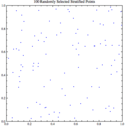
- stratified sampling
- moment matching
- conditional Monte Carlo
- and quasi random variables (in Quasi-Monte Carlo method)
For simulation with black-box models subset simulation and line sampling can also be used. Under these headings are a variety of specialized techniques; for example, particle transport simulations make extensive use of "weight windows" and "splitting/Russian roulette" techniques, which are a form of importance sampling.
Crude Monte Carlo simulation
Suppose one wants to compute with the random variable defined on the probability space . Monte Carlo does this by sampling i.i.d. copies of and then to estimate via the sample-mean estimator
Under further mild conditions such as , a central limit theorem will apply such that for large , the distribution of converges to a normal distribution with mean and standard error . Because the standard deviation only converges towards at the rate , implying one needs to increase the number of simulations () by a factor of to halve the standard deviation of , variance reduction methods are often useful for obtaining more precise estimates for without needing very large numbers of simulations.
Common Random Numbers (CRN)
The common random numbers variance reduction technique is a popular and useful variance reduction technique which applies when we are comparing two or more alternative configurations (of a system) instead of investigating a single configuration. CRN has also been called correlated sampling, matched streams or matched pairs.
CRN requires synchronization of the random number streams, which ensures that in addition to using the same random numbers to simulate all configurations, a specific random number used for a specific purpose in one configuration is used for exactly the same purpose in all other configurations. For example, in queueing theory, if we are comparing two different configurations of tellers in a bank, we would want the (random) time of arrival of the N-th customer to be generated using the same draw from a random number stream for both configurations.
Underlying principle of the CRN technique
Suppose and are the observations from the first and second configurations on the j-th independent replication.
We want to estimate
If we perform n replications of each configuration and let
then and is an unbiased estimator of .
And since the 's are independent identically distributed random variables,
In case of independent sampling, i.e., no common random numbers used then Cov(X1j, X2j) = 0. But if we succeed to induce an element of positive correlation between X1 and X2 such that Cov(X1j, X2j) > 0, it can be seen from the equation above that the variance is reduced.
It can also be observed that if the CRN induces a negative correlation, i.e., Cov(X1j, X2j) < 0, this technique can actually backfire, where the variance is increased and not decreased (as intended).[2]
See also
- Explained variance
- Regularization (mathematics)
References
- ↑ Botev, Z.; Ridder, A. (2017). "Variance Reduction". Wiley StatsRef: Statistics Reference Online. pp. 1–6. doi:10.1002/9781118445112.stat07975. ISBN 9781118445112.
- ↑ Hamrick, Jeff. "The Method of Common Random Numbers: An Example". http://demonstrations.wolfram.com/TheMethodOfCommonRandomNumbersAnExample/.
- Hammersley, J. M.; Handscomb, D. C. (1964). Monte Carlo Methods. London: Methuen. ISBN 0-416-52340-4.
- Kahn, H.; Marshall, A. W. (1953). "Methods of Reducing Sample Size in Monte Carlo Computations". Journal of the Operations Research Society of America 1 (5): 263–271. doi:10.1287/opre.1.5.263.
- MCNP — A General Monte Carlo N-Particle Transport Code, Version 5 Los Alamos Report LA-UR-03-1987
 |
