von Mises distribution

Short description: Probability distribution on the circle

von Mises

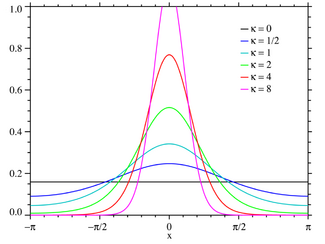
Probability density function The support is chosen to be [−π,π] with μ = 0
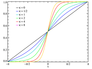
Cumulative distribution function The support is chosen to be [−π,π] with μ = 0
Parameters	[math]\displaystyle{ \mu }[/math] real [math]\displaystyle{ \kappa\gt 0 }[/math]
Support	[math]\displaystyle{ x\in }[/math] any interval of length 2π
PDF	[math]\displaystyle{ \frac{e^{\kappa\cos(x-\mu)}}{2\pi I_0(\kappa)} }[/math]
CDF	(not analytic – see text)
Mean	[math]\displaystyle{ \mu }[/math]
Median	[math]\displaystyle{ \mu }[/math]
Mode	[math]\displaystyle{ \mu }[/math]
Variance	[math]\displaystyle{ \textrm{var}(x)=1-I_1(\kappa)/I_0(\kappa) }[/math] (circular)
Entropy	[math]\displaystyle{ -\kappa\frac{I_1(\kappa)}{I_0(\kappa)}+\ln[2\pi I_0(\kappa)] }[/math] (differential)
CF	[math]\displaystyle{ \frac{I_{|t|}(\kappa)}{I_0(\kappa)}e^{i t \mu} }[/math]

In probability theory and directional statistics, the von Mises distribution (also known as the circular normal distribution or Tikhonov distribution) is a continuous probability distribution on the circle. It is a close approximation to the wrapped normal distribution, which is the circular analogue of the normal distribution. A freely diffusing angle [math]\displaystyle{ \theta }[/math] on a circle is a wrapped normally distributed random variable with an unwrapped variance that grows linearly in time. On the other hand, the von Mises distribution is the stationary distribution of a drift and diffusion process on the circle in a harmonic potential, i.e. with a preferred orientation. The von Mises distribution is the maximum entropy distribution for circular data when the real and imaginary parts of the first circular moment are specified. The von Mises distribution is a special case of the von Mises–Fisher distribution on the N-dimensional sphere.

Definition

The von Mises probability density function for the angle x is given by:

[math]\displaystyle{ f(x\mid\mu,\kappa)=\frac{\exp(\kappa\cos(x-\mu))}{2\pi I_0(\kappa)} }[/math]

where I₀([math]\displaystyle{ \kappa }[/math]) is the modified Bessel function of the first kind of order 0, with this scaling constant chosen so that the distribution sums to unity: [math]\displaystyle{ \int_{-\pi}^\pi \exp(\kappa\cos x)dx = {2\pi I_0(\kappa)}. }[/math]

The parameters μ and 1/[math]\displaystyle{ \kappa }[/math] are analogous to μ and σ² (the mean and variance) in the normal distribution:

• μ is a measure of location (the distribution is clustered around μ), and
• [math]\displaystyle{ \kappa }[/math] is a measure of concentration (a reciprocal measure of dispersion, so 1/[math]\displaystyle{ \kappa }[/math] is analogous to σ²).
  • If [math]\displaystyle{ \kappa }[/math] is zero, the distribution is uniform, and for small [math]\displaystyle{ \kappa }[/math], it is close to uniform.
  • If [math]\displaystyle{ \kappa }[/math] is large, the distribution becomes very concentrated about the angle μ with [math]\displaystyle{ \kappa }[/math] being a measure of the concentration. In fact, as [math]\displaystyle{ \kappa }[/math] increases, the distribution approaches a normal distribution in x  with mean μ and variance 1/[math]\displaystyle{ \kappa }[/math].

The probability density can be expressed as a series of Bessel functions

[math]\displaystyle{ f(x\mid\mu,\kappa) = \frac{1}{2\pi}\left(1+\frac{2}{I_0(\kappa)} \sum_{j=1}^\infty I_j(\kappa) \cos[j(x-\mu)]\right) }[/math]

where I_j(x) is the modified Bessel function of order j.

The cumulative distribution function is not analytic and is best found by integrating the above series. The indefinite integral of the probability density is:

[math]\displaystyle{ \Phi(x\mid\mu,\kappa)=\int f(t\mid\mu,\kappa)\,dt =\frac{1}{2\pi}\left(x + \frac{2}{I_0(\kappa)} \sum_{j=1}^\infty I_j(\kappa) \frac{\sin[j(x-\mu)]}{j}\right). }[/math]

The cumulative distribution function will be a function of the lower limit of integration x₀:

[math]\displaystyle{ F(x\mid\mu,\kappa)=\Phi(x\mid\mu,\kappa)-\Phi(x_0\mid\mu,\kappa).\, }[/math]

Moments

Further information: Circular mean

The moments of the von Mises distribution are usually calculated as the moments of the complex exponential z = e^ix rather than the angle x itself. These moments are referred to as circular moments. The variance calculated from these moments is referred to as the circular variance. The one exception to this is that the "mean" usually refers to the argument of the complex mean.

The nth raw moment of z is:

[math]\displaystyle{ m_n=\langle z^n\rangle=\int_\Gamma z^n\,f(x|\mu,\kappa)\,dx }[/math]

[math]\displaystyle{ = \frac{I_{|n|}(\kappa)}{I_0(\kappa)}e^{i n \mu} }[/math]

where the integral is over any interval [math]\displaystyle{ \Gamma }[/math] of length 2π. In calculating the above integral, we use the fact that zⁿ = cos(nx) + i sin(nx) and the Bessel function identity:

[math]\displaystyle{ I_n(\kappa)=\frac{1}{\pi}\int_0^\pi e^{\kappa\cos(x)}\cos(nx)\,dx. }[/math]

The mean of the complex exponential z  is then just

[math]\displaystyle{ m_1= \frac{I_1(\kappa)}{I_0(\kappa)}e^{i\mu} }[/math]

and the circular mean value of the angle x is then taken to be the argument μ. This is the expected or preferred direction of the angular random variables. The variance of z, or the circular variance of x is:

[math]\displaystyle{ \textrm{var}(x)= 1-E[\cos(x-\mu)] = 1-\frac{I_1(\kappa)}{I_0(\kappa)}. }[/math]

Limiting behavior

When [math]\displaystyle{ \kappa }[/math] is large, the distribution resembles a normal distribution. More specifically, for large positive real numbers [math]\displaystyle{ \kappa }[/math],

[math]\displaystyle{ f(x\mid\mu,\kappa) \approx \frac 1 {\sigma\sqrt{2\pi}} \exp\left[\dfrac{-(x-\mu)^2}{2\sigma^2}\right] }[/math]

where σ² = 1/[math]\displaystyle{ \kappa }[/math] and the difference between the left hand side and the right hand side of the approximation converges uniformly to zero as [math]\displaystyle{ \kappa }[/math] goes to infinity. Also, when [math]\displaystyle{ \kappa }[/math] is small, the probability density function resembles a uniform distribution:

[math]\displaystyle{ \lim_{\kappa\rightarrow 0}f(x\mid\mu,\kappa)=\mathrm{U}(x) }[/math]

where the interval for the uniform distribution [math]\displaystyle{ \mathrm{U}(x) }[/math] is the chosen interval of length [math]\displaystyle{ 2\pi }[/math] (i.e. [math]\displaystyle{ \mathrm{U}(x) = 1/(2\pi) }[/math] when [math]\displaystyle{ x }[/math] is in the interval and [math]\displaystyle{ \mathrm{U}(x)=0 }[/math] when [math]\displaystyle{ x }[/math] is not in the interval).

Estimation of parameters

A series of N measurements [math]\displaystyle{ z_n=e^{i\theta_n} }[/math] drawn from a von Mises distribution may be used to estimate certain parameters of the distribution. The average of the series [math]\displaystyle{ \overline{z} }[/math] is defined as

[math]\displaystyle{ \overline{z}=\frac{1}{N}\sum_{n=1}^N z_n }[/math]

and its expectation value will be just the first moment:

[math]\displaystyle{ \langle\overline{z}\rangle=\frac{I_1(\kappa)}{I_0(\kappa)}e^{i\mu}. }[/math]

In other words, [math]\displaystyle{ \overline{z} }[/math] is an unbiased estimator of the first moment. If we assume that the mean [math]\displaystyle{ \mu }[/math] lies in the interval [math]\displaystyle{ [-\pi,\pi] }[/math], then Arg[math]\displaystyle{ (\overline{z}) }[/math] will be a (biased) estimator of the mean [math]\displaystyle{ \mu }[/math].

Viewing the [math]\displaystyle{ z_n }[/math] as a set of vectors in the complex plane, the [math]\displaystyle{ \bar{R}^ 2 }[/math] statistic is the square of the length of the averaged vector:

[math]\displaystyle{ \bar{R}^ 2=\overline{z}\,\overline{z^*}=\left(\frac{1}{N}\sum_{n=1}^N \cos\theta_n\right)^2+\left(\frac{1}{N}\sum_{n=1}^N \sin\theta_n\right)^2 }[/math]

and its expectation value is

[math]\displaystyle{ \langle \bar{R}^2\rangle=\frac{1}{N}+\frac{N-1}{N}\,\frac{I_1(\kappa)^2}{I_0(\kappa)^2}. }[/math]

In other words, the statistic

[math]\displaystyle{ R_e^2=\frac{N}{N-1}\left(\bar{R}^2-\frac{1}{N}\right) }[/math]

will be an unbiased estimator of [math]\displaystyle{ \frac{I_1(\kappa)^2}{I_0(\kappa)^2}\, }[/math] and solving the equation [math]\displaystyle{ R_e=\frac{I_1(\kappa)}{I_0(\kappa)}\, }[/math] for [math]\displaystyle{ \kappa\, }[/math] will yield a (biased) estimator of [math]\displaystyle{ \kappa\, }[/math]. In analogy to the linear case, the solution to the equation [math]\displaystyle{ \bar{R}=\frac{I_1(\kappa)}{I_0(\kappa)}\, }[/math] will yield the maximum likelihood estimate of [math]\displaystyle{ \kappa\, }[/math] and both will be equal in the limit of large N. For approximate solution to [math]\displaystyle{ \kappa\, }[/math] refer to von Mises–Fisher distribution.

Distribution of the mean

The distribution of the sample mean [math]\displaystyle{ \overline{z} = \bar{R}e^{i\overline{\theta}} }[/math] for the von Mises distribution is given by:

[math]\displaystyle{ P(\bar{R},\bar{\theta})\,d\bar{R}\,d\bar{\theta}=\frac{1}{ (2\pi I_0(\kappa))^N}\int_\Gamma \prod_{n=1}^N \left( e^{\kappa\cos(\theta_n-\mu)} d\theta_n\right) = \frac{e^{\kappa N\bar{R}\cos(\bar{\theta}-\mu)}}{I_0(\kappa)^N}\left(\frac{1}{(2\pi)^N}\int_\Gamma \prod_{n=1}^N d\theta_n\right) }[/math]

where N is the number of measurements and [math]\displaystyle{ \Gamma\, }[/math] consists of intervals of [math]\displaystyle{ 2\pi }[/math] in the variables, subject to the constraint that [math]\displaystyle{ \bar{R} }[/math] and [math]\displaystyle{ \bar{\theta} }[/math] are constant, where [math]\displaystyle{ \bar{R} }[/math] is the mean resultant:

[math]\displaystyle{ \bar{R}^2=|\bar{z}|^2= \left(\frac{1}{N}\sum_{n=1}^N \cos(\theta_n) \right)^2 + \left(\frac{1}{N}\sum_{n=1}^N \sin(\theta_n) \right)^2 }[/math]

and [math]\displaystyle{ \overline{\theta} }[/math] is the mean angle:

[math]\displaystyle{ \overline{\theta}=\mathrm{Arg}(\overline{z}). \, }[/math]

Note that product term in parentheses is just the distribution of the mean for a circular uniform distribution.

This means that the distribution of the mean direction [math]\displaystyle{ \mu }[/math] of a von Mises distribution [math]\displaystyle{ VM(\mu, \kappa) }[/math] is a von Mises distribution [math]\displaystyle{ VM(\mu, \bar{R}N\kappa) }[/math], or, equivalently, [math]\displaystyle{ VM(\mu, R\kappa) }[/math].

Entropy

By definition, the information entropy of the von Mises distribution is

[math]\displaystyle{ H = -\int_\Gamma f(\theta;\mu,\kappa)\,\ln(f(\theta;\mu,\kappa))\,d\theta\, }[/math]

where [math]\displaystyle{ \Gamma }[/math] is any interval of length [math]\displaystyle{ 2\pi }[/math]. The logarithm of the density of the Von Mises distribution is straightforward:

[math]\displaystyle{ \ln(f(\theta;\mu,\kappa))=-\ln(2\pi I_0(\kappa))+ \kappa \cos(\theta)\, }[/math]

The characteristic function representation for the Von Mises distribution is:

[math]\displaystyle{ f(\theta;\mu,\kappa) =\frac{1}{2\pi}\left(1+2\sum_{n=1}^\infty\phi_n\cos(n\theta)\right) }[/math]

where [math]\displaystyle{ \phi_n= I_{|n|}(\kappa)/I_0(\kappa) }[/math]. Substituting these expressions into the entropy integral, exchanging the order of integration and summation, and using the orthogonality of the cosines, the entropy may be written:

[math]\displaystyle{ H = \ln(2\pi I_0(\kappa))-\kappa\phi_1 = \ln(2\pi I_0(\kappa))-\kappa\frac{I_1(\kappa)}{I_0(\kappa)} }[/math]

For [math]\displaystyle{ \kappa=0 }[/math], the von Mises distribution becomes the circular uniform distribution and the entropy attains its maximum value of [math]\displaystyle{ \ln(2\pi) }[/math].

Notice that the Von Mises distribution maximizes the entropy when the real and imaginary parts of the first circular moment are specified or, equivalently, the circular mean and circular variance are specified.

See also

• Bivariate von Mises distribution
• Directional statistics
• Von Mises–Fisher distribution
• Kent distribution

Further reading

• Abramowitz, M. and Stegun, I. A. (ed.), Handbook of Mathematical Functions, National Bureau of Standards, 1964; reprinted Dover Publications, 1965. ISBN 0-486-61272-4
• "Algorithm AS 86: The von Mises Distribution Function", Mardia, Applied Statistics, 24, 1975 (pp. 268–272).
• "Algorithm 518, Incomplete Bessel Function I0: The von Mises Distribution", Hill, ACM Transactions on Mathematical Software, Vol. 3, No. 3, September 1977, Pages 279–284.
• Best, D. and Fisher, N. (1979). Efficient simulation of the von Mises distribution. Applied Statistics, 28, 152–157.
• Evans, M., Hastings, N., and Peacock, B., "von Mises Distribution". Ch. 41 in Statistical Distributions, 3rd ed. New York. Wiley 2000.
• Fisher, Nicholas I., Statistical Analysis of Circular Data. New York. Cambridge 1993.
• "Statistical Distributions", 2nd. Edition, Evans, Hastings, and Peacock, John Wiley and Sons, 1993, (chapter 39). ISBN 0-471-55951-2
• Borradaile, Graham (2003). Statistics of Earth Science Data. Springer. ISBN 978-3-540-43603-4. https://books.google.com/books?id=R3GpDglVOSEC. Retrieved 31 Dec 2009.

References

- ↑ Risken, H. (1989). The Fokker–Planck Equation. Springer. ISBN 978-3-540-61530-9.
- ↑ 2.0 2.1 Mardia, Kantilal; Jupp, Peter E. (1999). Directional Statistics. Wiley. ISBN 978-0-471-95333-3.
- ↑ see Abramowitz and Stegun §9.6.34
- ↑ See Abramowitz and Stegun §9.6.19
- ↑ de Abreu, Giuseppe Thadeu Freitas (2008). "On the Generation of Tikhonov Variates". IEEE Transactions on Communications 56 (7): 1157–1168. doi:10.1109/TCOMM.2008.060510.
- ↑ [On the Generation of Tikhonov Random Variates]. YouTube (Video). [The Wireless Channel]. 2025-03-19. Retrieved 2025-03-21.
- ↑ Mardia, K. V.; Jupp, P. E. (2000). "Directional Statistics". Wiley Series in Probability and Statistics. Chichester: John Wiley & Sons. ISBN 978-0-471-95333-3. p. 36.
- ↑ Borradaile, G. J. (2003). Statistics of earth science data : their distribution in time, space, and orientation. Springer. ISBN 978-3-662-05223-5.
- ↑ Kutil, Rade (August 2012). "Biased and unbiased estimation of the circular mean resultant length and its variance.". Statistics: A Journal of Theoretical and Applied Statistics 46 (4): 549–561. doi:10.1080/02331888.2010.543463. https://www.researchgate.net/publication/233474043.
- ↑ 10.0 10.1 Jammalamadaka, S. Rao; Sengupta, A. (2001). Topics in Circular Statistics. World Scientific Publishing Company. ISBN 978-981-02-3778-3.
- ↑ Jammalamadaka, S. Rao; SenGupta, A. (2001). Topics in circular statistics. New Jersey: World Scientific. ISBN 981-02-3778-2. https://books.google.com/books?id=sKqWMGqQXQkC&q=Jammalamadaka+Topics+in+circular. Retrieved 2011-05-15.