Wrapped Cauchy distribution

Wrapped Cauchy

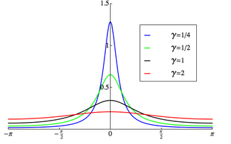
Probability density function The support is chosen to be [-π,π)
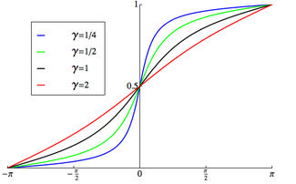
Cumulative distribution function The support is chosen to be [-π,π)
Parameters	[math]\displaystyle{ \mu }[/math] Real [math]\displaystyle{ \gamma\gt 0 }[/math]
Support	[math]\displaystyle{ -\pi\le\theta\lt \pi }[/math]
PDF	[math]\displaystyle{ \frac{1}{2\pi}\,\frac{\sinh(\gamma)}{\cosh(\gamma)-\cos(\theta-\mu)} }[/math]
CDF	[math]\displaystyle{ \, }[/math]
Mean	[math]\displaystyle{ \mu }[/math] (circular)
Variance	[math]\displaystyle{ 1-e^{-\gamma} }[/math] (circular)
Entropy	[math]\displaystyle{ \ln(2\pi(1-e^{-2\gamma})) }[/math] (differential)
CF	[math]\displaystyle{ e^{in\mu-|n|\gamma} }[/math]

In probability theory and directional statistics, a wrapped Cauchy distribution is a wrapped probability distribution that results from the "wrapping" of the Cauchy distribution around the unit circle. The Cauchy distribution is sometimes known as a Lorentzian distribution, and the wrapped Cauchy distribution may sometimes be referred to as a wrapped Lorentzian distribution.

The wrapped Cauchy distribution is often found in the field of spectroscopy where it is used to analyze diffraction patterns (e.g. see Fabry–Pérot interferometer).

Description

The probability density function of the wrapped Cauchy distribution is:

[math]\displaystyle{ f_{WC}(\theta;\mu,\gamma)=\sum_{n=-\infty}^\infty \frac{\gamma}{\pi(\gamma^2+(\theta-\mu+2\pi n)^2)}\qquad -\pi\lt \theta\lt \pi }[/math]

where [math]\displaystyle{ \gamma }[/math] is the scale factor and [math]\displaystyle{ \mu }[/math] is the peak position of the "unwrapped" distribution. Expressing the above pdf in terms of the characteristic function of the Cauchy distribution yields:

[math]\displaystyle{ f_{WC}(\theta;\mu,\gamma)=\frac{1}{2\pi}\sum_{n=-\infty}^\infty e^{in(\theta-\mu)-|n|\gamma} =\frac{1}{2\pi}\,\,\frac{\sinh\gamma}{\cosh\gamma-\cos(\theta-\mu)} }[/math]

The PDF may also be expressed in terms of the circular variable z = e^iθ and the complex parameter ζ = e^i(μ+iγ)

[math]\displaystyle{ f_{WC}(z;\zeta)=\frac{1}{2\pi}\,\,\frac{1-|\zeta|^2}{|z-\zeta|^2} }[/math]

where, as shown below, ζ = ⟨z⟩.

In terms of the circular variable [math]\displaystyle{ z=e^{i\theta} }[/math] the circular moments of the wrapped Cauchy distribution are the characteristic function of the Cauchy distribution evaluated at integer arguments:

[math]\displaystyle{ \langle z^n\rangle=\int_\Gamma e^{in\theta}\,f_{WC}(\theta;\mu,\gamma)\,d\theta = e^{i n \mu-|n|\gamma}. }[/math]

where [math]\displaystyle{ \Gamma\, }[/math] is some interval of length [math]\displaystyle{ 2\pi }[/math]. The first moment is then the average value of z, also known as the mean resultant, or mean resultant vector:

[math]\displaystyle{ \langle z \rangle=e^{i\mu-\gamma} }[/math]

The mean angle is

[math]\displaystyle{ \langle \theta \rangle=\mathrm{Arg}\langle z \rangle = \mu }[/math]

and the length of the mean resultant is

[math]\displaystyle{ R=|\langle z \rangle| = e^{-\gamma} }[/math]

yielding a circular variance of 1 − R.

Estimation of parameters

A series of N measurements [math]\displaystyle{ z_n=e^{i\theta_n} }[/math] drawn from a wrapped Cauchy distribution may be used to estimate certain parameters of the distribution. The average of the series [math]\displaystyle{ \overline{z} }[/math] is defined as

[math]\displaystyle{ \overline{z}=\frac{1}{N}\sum_{n=1}^N z_n }[/math]

and its expectation value will be just the first moment:

[math]\displaystyle{ \langle\overline{z}\rangle=e^{i\mu-\gamma} }[/math]

In other words, [math]\displaystyle{ \overline{z} }[/math] is an unbiased estimator of the first moment. If we assume that the peak position [math]\displaystyle{ \mu }[/math] lies in the interval [math]\displaystyle{ [-\pi,\pi) }[/math], then Arg[math]\displaystyle{ (\overline{z}) }[/math] will be a (biased) estimator of the peak position [math]\displaystyle{ \mu }[/math].

Viewing the [math]\displaystyle{ z_n }[/math] as a set of vectors in the complex plane, the [math]\displaystyle{ \overline{R}^2 }[/math] statistic is the length of the averaged vector:

[math]\displaystyle{ \overline{R}^2=\overline{z}\,\overline{z^*}=\left(\frac{1}{N}\sum_{n=1}^N \cos\theta_n\right)^2+\left(\frac{1}{N}\sum_{n=1}^N \sin\theta_n\right)^2 }[/math]

and its expectation value is

[math]\displaystyle{ \langle \overline{R}^2\rangle=\frac{1}{N}+\frac{N-1}{N}e^{-2\gamma}. }[/math]

In other words, the statistic

[math]\displaystyle{ R_e^2=\frac{N}{N-1}\left(\overline{R}^2-\frac{1}{N}\right) }[/math]

will be an unbiased estimator of [math]\displaystyle{ e^{-2\gamma} }[/math], and [math]\displaystyle{ \ln(1/R_e^2)/2 }[/math] will be a (biased) estimator of [math]\displaystyle{ \gamma }[/math].

Entropy

The information entropy of the wrapped Cauchy distribution is defined as:

[math]\displaystyle{ H = -\int_\Gamma f_{WC}(\theta;\mu,\gamma)\,\ln(f_{WC}(\theta;\mu,\gamma))\,d\theta }[/math]

where [math]\displaystyle{ \Gamma }[/math] is any interval of length [math]\displaystyle{ 2\pi }[/math]. The logarithm of the density of the wrapped Cauchy distribution may be written as a Fourier series in [math]\displaystyle{ \theta\, }[/math]:

[math]\displaystyle{ \ln(f_{WC}(\theta;\mu,\gamma))=c_0+2\sum_{m=1}^\infty c_m \cos(m\theta) }[/math]

where

[math]\displaystyle{ c_m=\frac{1}{2\pi}\int_\Gamma \ln\left(\frac{\sinh\gamma}{2\pi(\cosh\gamma-\cos\theta)}\right)\cos(m \theta)\,d\theta }[/math]

which yields:

[math]\displaystyle{ c_0 = \ln\left(\frac{1-e^{-2\gamma}}{2\pi}\right) }[/math]

(c.f. Gradshteyn and Ryzhik 4.224.15) and

[math]\displaystyle{ c_m=\frac{e^{-m\gamma}}{m}\qquad \mathrm{for}\,m\gt 0 }[/math]

(c.f. Gradshteyn and Ryzhik 4.397.6). The characteristic function representation for the wrapped Cauchy distribution in the left side of the integral is:

[math]\displaystyle{ f_{WC}(\theta;\mu,\gamma) =\frac{1}{2\pi}\left(1+2\sum_{n=1}^\infty\phi_n\cos(n\theta)\right) }[/math]

where [math]\displaystyle{ \phi_n= e^{-|n|\gamma} }[/math]. Substituting these expressions into the entropy integral, exchanging the order of integration and summation, and using the orthogonality of the cosines, the entropy may be written:

[math]\displaystyle{ H = -c_0-2\sum_{m=1}^\infty \phi_m c_m = -\ln\left(\frac{1-e^{-2\gamma}}{2\pi}\right)-2\sum_{m=1}^\infty \frac{e^{-2n\gamma}}{n} }[/math]

The series is just the Taylor expansion for the logarithm of [math]\displaystyle{ (1-e^{-2\gamma}) }[/math] so the entropy may be written in closed form as:

[math]\displaystyle{ H=\ln(2\pi(1-e^{-2\gamma}))\, }[/math]

Circular Cauchy distribution

If X is Cauchy distributed with median μ and scale parameter γ, then the complex variable

[math]\displaystyle{ Z = \frac{X - i}{X+i} }[/math]

has unit modulus and is distributed on the unit circle with density:

[math]\displaystyle{ f_{CC}(\theta,\mu,\gamma)= \frac{1}{2\pi } \frac{1 - |\zeta|^2}{|e^{i \theta} - \zeta|^2} }[/math]

where

[math]\displaystyle{ \zeta = \frac{\psi - i}{\psi + i} }[/math]

and ψ expresses the two parameters of the associated linear Cauchy distribution for x as a complex number:

[math]\displaystyle{ \psi=\mu+i\gamma\, }[/math]

It can be seen that the circular Cauchy distribution has the same functional form as the wrapped Cauchy distribution in z and ζ (i.e. f_WC(z,ζ)). The circular Cauchy distribution is a reparameterized wrapped Cauchy distribution:

[math]\displaystyle{ f_{CC}(\theta,m,\gamma)=f_{WC}\left(e^{i \theta},\, \frac{m+i \gamma -i}{m+i\gamma+i}\right) }[/math]

The distribution [math]\displaystyle{ f_{CC}(\theta; \mu,\gamma) }[/math] is called the circular Cauchy distribution (also the complex Cauchy distribution) with parameters μ and γ. (See also McCullagh's parametrization of the Cauchy distributions and Poisson kernel for related concepts.)

The circular Cauchy distribution expressed in complex form has finite moments of all orders

[math]\displaystyle{ \operatorname{E}[Z^n] = \zeta^n, \quad \operatorname{E}[\bar Z^n] = \bar\zeta^n }[/math]

for integer n ≥ 1. For |φ| < 1, the transformation

[math]\displaystyle{ U(z, \phi) = \frac{z - \phi}{1 - \bar \phi z} }[/math]

is holomorphic on the unit disk, and the transformed variable U(Z, φ) is distributed as complex Cauchy with parameter U(ζ, φ).

Given a sample z₁, ..., z_n of size n > 2, the maximum-likelihood equation

[math]\displaystyle{ n^{-1} U \left(z, \hat\zeta \right) = n^{-1} \sum U \left(z_j, \hat\zeta \right) = 0 }[/math]

can be solved by a simple fixed-point iteration:

[math]\displaystyle{ \zeta^{(r+1)} = U \left(n^{-1} U(z, \zeta^{(r)}), \, - \zeta^{(r)} \right)\, }[/math]

starting with ζ⁽⁰⁾ = 0. The sequence of likelihood values is non-decreasing, and the solution is unique for samples containing at least three distinct values.

The maximum-likelihood estimate for the median ([math]\displaystyle{ \hat\mu }[/math]) and scale parameter ([math]\displaystyle{ \hat\gamma }[/math]) of a real Cauchy sample is obtained by the inverse transformation:

[math]\displaystyle{ \hat\mu \pm i\hat\gamma = i\frac{1+\hat\zeta}{1-\hat\zeta}. }[/math]

For n ≤ 4, closed-form expressions are known for [math]\displaystyle{ \hat\zeta }[/math]. The density of the maximum-likelihood estimator at t in the unit disk is necessarily of the form:

[math]\displaystyle{ \frac{1}{4\pi}\frac{p_n(\chi(t, \zeta))}{(1 - |t|^2)^2} , }[/math]

where

[math]\displaystyle{ \chi(t, \zeta) = \frac{ |t - \zeta|^2}{4(1 - |t|^2)(1 - |\zeta|^2)} }[/math].

Formulae for p₃ and p₄ are available.

See also

• Wrapped distribution
• Dirac comb
• Wrapped normal distribution
• Circular uniform distribution
• McCullagh's parametrization of the Cauchy distributions

References

• Borradaile, Graham (2003). Statistics of Earth Science Data. Springer. ISBN 978-3-540-43603-4. https://books.google.com/books?id=R3GpDglVOSEC. Retrieved 31 Dec 2009. 
• Fisher, N. I. (1996). Statistical Analysis of Circular Data. Cambridge University Press. ISBN 978-0-521-56890-6. https://books.google.com/books?id=IIpeevaNH88C&q=%22circular+variance%22+fisher. Retrieved 2010-02-09.

References

- ↑ 1.0 1.1 Mardia, Kantilal; Jupp, Peter E. (1999). Directional Statistics. Wiley. ISBN 978-0-471-95333-3.
- ↑ 2.0 2.1 (in en) Table of Integrals, Series, and Products (7 ed.). Academic Press, Inc.. February 2007. ISBN 0-12-373637-4.
- ↑ 3.0 3.1 3.2 McCullagh, Peter (June 1992). "Conditional inference and Cauchy models". Biometrika 79 (2): 247–259. doi:10.1093/biomet/79.2.247. http://www.stat.uchicago.edu/~pmcc/pubs/paper18.pdf. Retrieved 26 January 2016.
- ↑ K.V. Mardia (1972). Statistics of Directional Data. Academic Press.
- ↑ J. Copas (1975). "On the unimodality of the likelihood function for the Cauchy distribution". Biometrika 62 (3): 701–704. doi:10.1093/biomet/62.3.701.
- ↑ Ferguson, Thomas S. (1978). "Maximum Likelihood Estimates of the Parameters of the Cauchy Distribution for Samples of Size 3 and 4". Journal of the American Statistical Association 73 (361): 211–213. doi:10.1080/01621459.1978.10480031.
- ↑ P. McCullagh (1996). "Möbius transformation and Cauchy parameter estimation.". Annals of Statistics 24 (2): 786–808. doi:10.1214/aos/1032894465.