Logarithmic distribution
|
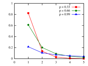
Probability mass function The function is only defined at integer values. The connecting lines are merely guides for the eye. | |||
|
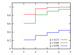
Cumulative distribution function | |||
| Parameters | [math]\displaystyle{ 0 \lt p \lt 1 }[/math] | ||
|---|---|---|---|
| Support | [math]\displaystyle{ k \in \{1,2,3,\ldots\} }[/math] | ||
| pmf | [math]\displaystyle{ \frac{-1}{\ln(1-p)} \frac{p^k}{k} }[/math] | ||
| CDF | [math]\displaystyle{ 1 + \frac{\Beta(p;k+1,0)}{\ln(1-p)} }[/math] | ||
| Mean | [math]\displaystyle{ \frac{-1}{\ln(1-p)} \frac{p}{1-p} }[/math] | ||
| Mode | [math]\displaystyle{ 1 }[/math] | ||
| Variance | [math]\displaystyle{ - \frac{p^2 + p\ln(1-p)}{(1-p)^2(\ln(1-p))^2} }[/math] | ||
| MGF | [math]\displaystyle{ \frac{\ln(1 - pe^t)}{\ln(1-p)}\text{ for }t \lt -\ln p }[/math] | ||
| CF | [math]\displaystyle{ \frac{\ln(1 - pe^{it})}{\ln(1-p)} }[/math] | ||
| PGF | [math]\displaystyle{ \frac{\ln(1-pz)}{\ln(1-p)}\text{ for }|z| \lt \frac{1}{p} }[/math] | ||
In probability and statistics, the logarithmic distribution (also known as the logarithmic series distribution or the log-series distribution) is a discrete probability distribution derived from the Maclaurin series expansion
- [math]\displaystyle{ -\ln(1-p) = p + \frac{p^2}{2} + \frac{p^3}{3} + \cdots. }[/math]
From this we obtain the identity
- [math]\displaystyle{ \sum_{k=1}^{\infty} \frac{-1}{\ln(1-p)} \; \frac{p^k}{k} = 1. }[/math]
This leads directly to the probability mass function of a Log(p)-distributed random variable:
- [math]\displaystyle{ f(k) = \frac{-1}{\ln(1-p)} \; \frac{p^k}{k} }[/math]
for k ≥ 1, and where 0 < p < 1. Because of the identity above, the distribution is properly normalized.
The cumulative distribution function is
- [math]\displaystyle{ F(k) = 1 + \frac{\Beta(p; k+1,0)}{\ln(1-p)} }[/math]
where B is the incomplete beta function.
A Poisson compounded with Log(p)-distributed random variables has a negative binomial distribution. In other words, if N is a random variable with a Poisson distribution, and Xi, i = 1, 2, 3, ... is an infinite sequence of independent identically distributed random variables each having a Log(p) distribution, then
- [math]\displaystyle{ \sum_{i=1}^N X_i }[/math]
has a negative binomial distribution. In this way, the negative binomial distribution is seen to be a compound Poisson distribution.
R. A. Fisher described the logarithmic distribution in a paper that used it to model relative species abundance.[1]
See also
- Poisson distribution (also derived from a Maclaurin series)
References
- ↑ Fisher, R. A.; Corbet, A. S.; Williams, C. B. (1943). "The Relation Between the Number of Species and the Number of Individuals in a Random Sample of an Animal Population". Journal of Animal Ecology 12 (1): 42–58. doi:10.2307/1411. http://www.math.mcgill.ca/~dstephens/556/Papers/Fisher1943.pdf.
Further reading
- Johnson, Norman Lloyd; Kemp, Adrienne W; Kotz, Samuel (2005). "Chapter 7: Logarithmic and Lagrangian distributions". Univariate discrete distributions (3 ed.). John Wiley & Sons. ISBN 978-0-471-27246-5.
- Weisstein, Eric W.. "Log-Series Distribution". http://mathworld.wolfram.com/Log-SeriesDistribution.html.
 |


